Data classes

Environmental Data Analysis and Visualization

https://mrne222-sp25.github.io/website/

Data classes

We’ve talked about types so far, next we’ll introduce the concept of classes

Vectors are like Lego building blocks
We stick them together to build more complicated constructs, e.g. representations of data
The class attribute relates to the S3 class of an object which determines its behaviour
- You don’t need to worry about what S3 classes really mean, but you can read more about it here if you’re curious
Examples: factors, dates, and data frames

Factors

R uses factors to handle categorical variables, variables that have a fixed and known set of possible values

x <- factor(c("BS", "MS", "PhD", "MS"))
x

[1] BS  MS  PhD MS 
Levels: BS MS PhD

typeof(x)

[1] "integer"

class(x)

[1] "factor"

More on factors

We can think of factors like character (level labels) and an integer (level numbers) glued together

glimpse(x)

 Factor w/ 3 levels "BS","MS","PhD": 1 2 3 2

as.integer(x)

[1] 1 2 3 2

Dates

y <- as.Date("2020-01-01")
y

[1] "2020-01-01"

typeof(y)

[1] "double"

class(y)

[1] "Date"

More on dates

We can think of dates like an integer (the number of days since the origin, 1 Jan 1970) and an integer (the origin) glued together

as.integer(y)

[1] 18262

as.integer(y) / 365 # roughly 50 yrs

[1] 50.03288

Data frames

We can think of data frames like like vectors of equal length glued together

df <- data.frame(x = 1:2, y = 3:4)
df

  x y
1 1 3
2 2 4

typeof(df)

[1] "list"

class(df)

[1] "data.frame"

Lists

Lists are a generic vector container. Vectors of any type can go in them.

l <- list(
  x = 1:4,
  y = c("hi", "hello", "jello"),
  z = c(TRUE, FALSE)
)
l

$x
[1] 1 2 3 4

$y
[1] "hi"    "hello" "jello"

$z
[1]  TRUE FALSE

Lists and data frames

A data frame is a special list containing vectors of equal length
When we use the pull() function, we extract a vector from the data frame

df

  x y
1 1 3
2 2 4

df |>
  pull(y)

[1] 3 4

Working with factors

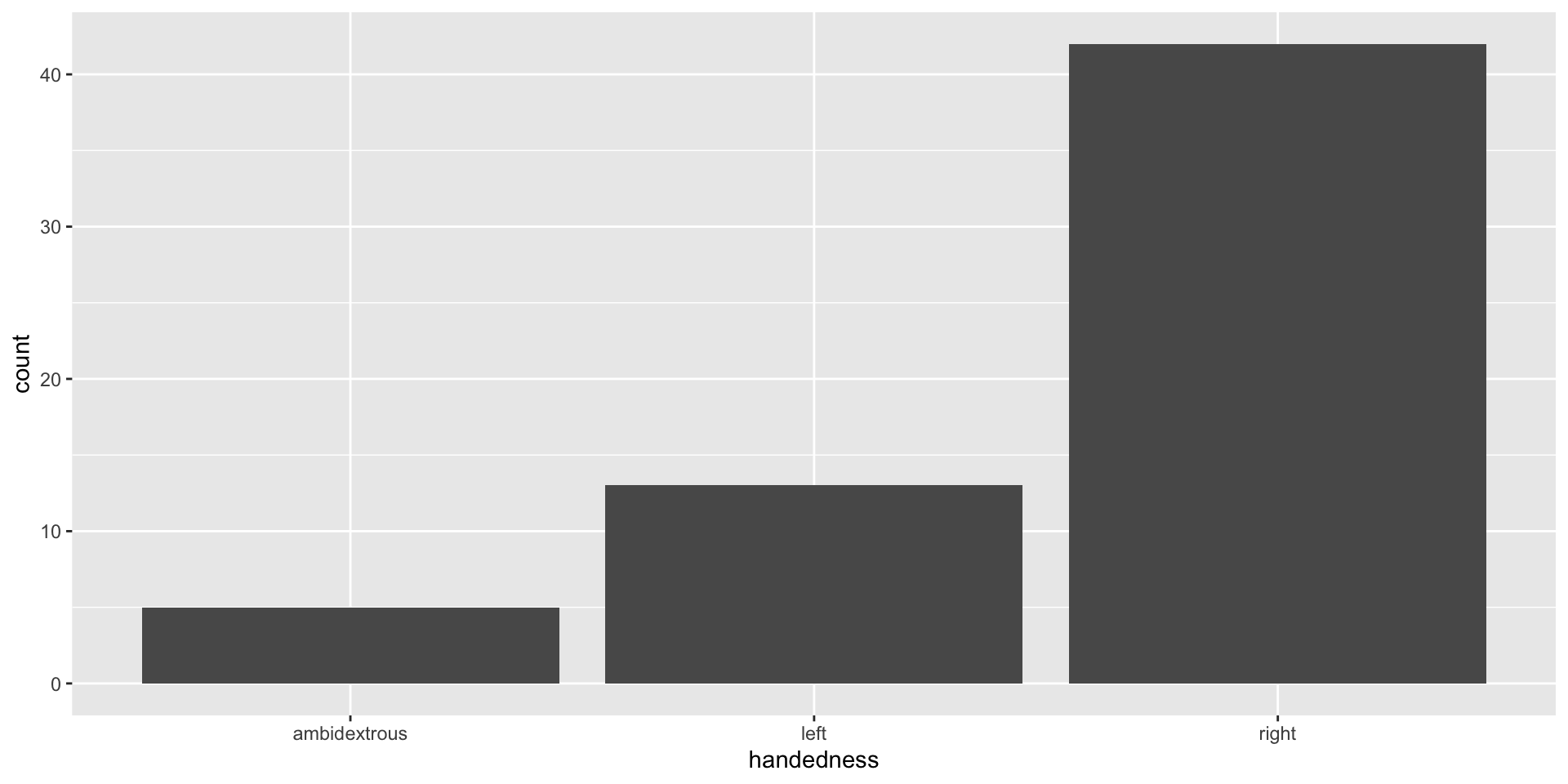
The data are read data in as character strings

glimpse(cat_lovers)

Rows: 60
Columns: 3
$ name           <chr> "Bernice Warren", "Woodrow Stone", "Willie Bass", "Tyro…
$ number_of_cats <chr> "0", "0", "1", "3", "3", "2", "1", "1", "0", "0", "0", …
$ handedness     <chr> "left", "left", "left", "left", "left", "left", "left",…

Defaut plot of “handedness” counts

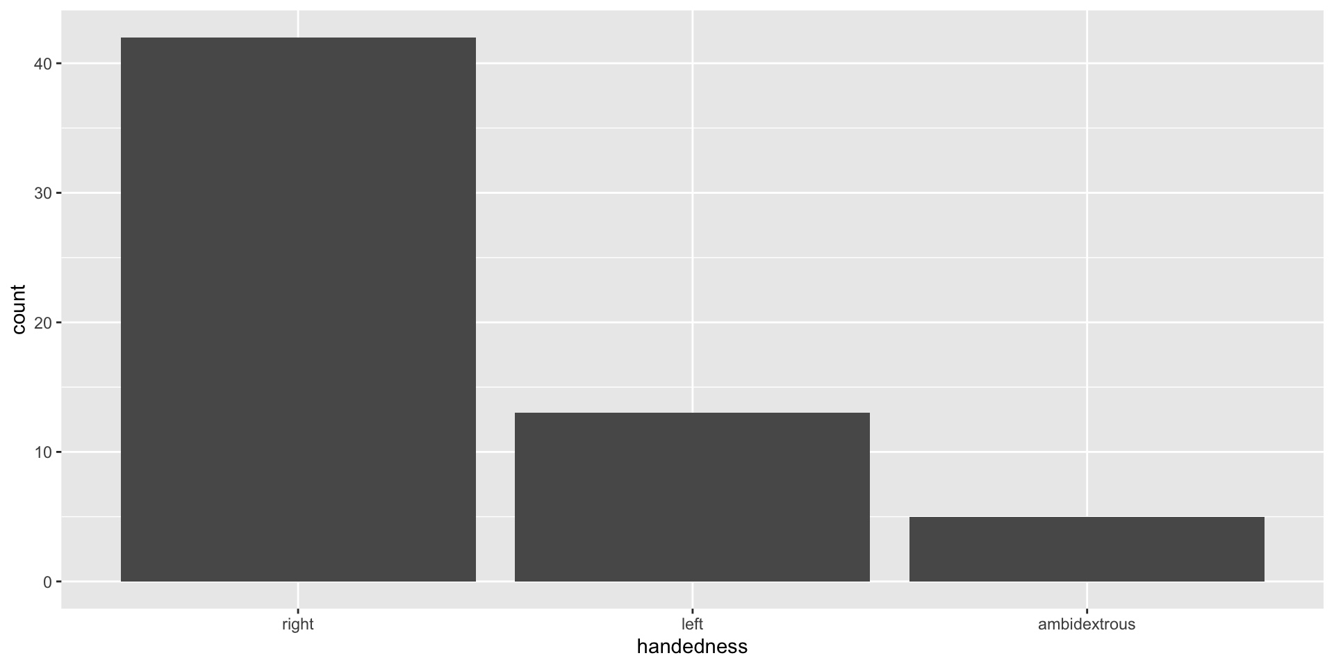
ggplot(cat_lovers, mapping = aes(x = handedness)) +
  geom_bar()

Use the forcats package to manipulate factors

cat_lovers |>
  mutate(handedness = fct_infreq(handedness)) |> 
  ggplot(aes(x = handedness)) +
  geom_bar()

Come for the functionality

… stay for the logo

Why use factors?

Factors are useful when you have true categorical data and you want to override the ordering of character vectors to improve display
They are also useful in modeling scenarios
The forcats package provides a suite of useful tools that solve common problems with factors

AE-08

AE 08 - data types and classes > forcats.Rmd

Working with dates

Make a date

lubridate is the tidyverse-friendly package that makes dealing with dates easier
It’s not one of the core tidyverse packages: it’s installed with install.packages("tidyverse) but it’s not loaded with it and needs to be explicitly loaded with library(lubridate)

We’re just going to scratch the surface of working with dates in R here…

Dates and times in R

A date. Tibbles print this as <date>.
A time within a day. Tibbles print this as <time>.
A date-time is a date plus a time: it uniquely identifies an instant in time (typically to the nearest second). Tibbles print this as <dttm>. Elsewhere in R these are called POSIXct, but I don’t think that’s a very useful name.

When you read in data, check data types

flats <- read_csv("data/flats_sub_2015.csv")
flats

# A tibble: 672 × 10
   date   time     datetime depth_m salinity_ppt    ph do_mg_l turb_ntu chl_ug_l
   <chr>  <time>   <chr>      <dbl>        <dbl> <dbl>   <dbl>    <dbl>    <dbl>
 1 7/1/15 00:00:24 7/1/15 …   0.741         0.12  8.53   10.2       1.9      4.3
 2 7/1/15 00:15:24 7/1/15 …   0.706         0.12  8.45    9.91      2        3.8
 3 7/1/15 00:30:24 7/1/15 …   0.687         0.12  8.38    9.68      1.9      4.3
 4 7/1/15 00:45:24 7/1/15 …   0.684         0.12  8.29    9.47      2        4.3
 5 7/1/15 01:00:23 7/1/15 …   0.73          0.12  7.94    8.49      6.1     10.7
 6 7/1/15 01:15:24 7/1/15 …   0.683         0.12  7.67    7.9       6.1     11.6
 7 7/1/15 01:30:24 7/1/15 …   0.664         0.12  7.75    8.07      5.3     20.7
 8 7/1/15 01:45:24 7/1/15 …   0.659         0.12  7.78    8.02      4.8      5.5
 9 7/1/15 02:00:24 7/1/15 …   0.724         0.12  7.81    8         4.5      5.1
10 7/1/15 02:15:24 7/1/15 …   0.782         0.12  7.76    7.88      3.9     27.4
# ℹ 662 more rows
# ℹ 1 more variable: t_c <dbl>

When you read in data, check data types

flats <- read_csv("data/flats_sub_2015.csv") |> 
  print(n = 1)

# A tibble: 672 × 10
  date   time   datetime    depth_m salinity_ppt    ph do_mg_l turb_ntu chl_ug_l
  <chr>  <time> <chr>         <dbl>        <dbl> <dbl>   <dbl>    <dbl>    <dbl>
1 7/1/15 00'24" 7/1/15 0:00   0.741         0.12  8.53    10.2      1.9      4.3
# ℹ 671 more rows
# ℹ 1 more variable: t_c <dbl>

date was read in as a character
time was read in as a time
datetime was read in as a character

Why is this a problem?

ggplot(flats, aes(x = datetime, y = depth_m)) +
  geom_point()

Using the `lubridate` functions

Lubridate works out the date/time format once you specify the order of components
- Identify the order in which year, month, and day appear in your dates
- Then arrange “y”, “m”, and “d” (year, month, day) and “h”, “m”, and “s” (hour, minute, second) in the same order.
- That gives you the name of the lubridate function that will parse your date.
- The resulting output is always in yyyy-mm-dd format

Using the `lubridate` functions

ymd("2017-01-31")

[1] "2017-01-31"

mdy("January 31st, 2017")

[1] "2017-01-31"

dmy("31-Jan-2017")

[1] "2017-01-31"

ymd_hms("2017-01-31 3:15:00")

[1] "2017-01-31 03:15:00 UTC"

ymd_hm("2017-01-31 3:15")

[1] "2017-01-31 03:15:00 UTC"

ymd(20170131)

[1] "2017-01-31"

Coerce `flats` data into dates and datetimes

flats |> 
  mutate(datetime = mdy_hm(datetime),
         date = mdy(date))

# A tibble: 672 × 10
   date       time     datetime            depth_m salinity_ppt    ph do_mg_l
   <date>     <time>   <dttm>                <dbl>        <dbl> <dbl>   <dbl>
 1 2015-07-01 00:00:24 2015-07-01 00:00:00   0.741         0.12  8.53   10.2 
 2 2015-07-01 00:15:24 2015-07-01 00:15:00   0.706         0.12  8.45    9.91
 3 2015-07-01 00:30:24 2015-07-01 00:30:00   0.687         0.12  8.38    9.68
 4 2015-07-01 00:45:24 2015-07-01 00:45:00   0.684         0.12  8.29    9.47
 5 2015-07-01 01:00:23 2015-07-01 01:00:00   0.73          0.12  7.94    8.49
 6 2015-07-01 01:15:24 2015-07-01 01:15:00   0.683         0.12  7.67    7.9 
 7 2015-07-01 01:30:24 2015-07-01 01:30:00   0.664         0.12  7.75    8.07
 8 2015-07-01 01:45:24 2015-07-01 01:45:00   0.659         0.12  7.78    8.02
 9 2015-07-01 02:00:24 2015-07-01 02:00:00   0.724         0.12  7.81    8   
10 2015-07-01 02:15:24 2015-07-01 02:15:00   0.782         0.12  7.76    7.88
# ℹ 662 more rows
# ℹ 3 more variables: turb_ntu <dbl>, chl_ug_l <dbl>, t_c <dbl>

Now it knows the dates are actually datetimes

flats |> 
  mutate(datetime = mdy_hm(datetime),
         date = mdy(date)) |> 
  ggplot(aes(x = datetime, y = depth_m)) +
    geom_line() +
    labs(x = "", y = "Depth (m)") +
    theme_minimal()

What if your data contain year, month, day, etc. in separate columns?

flats2 <- flats |>
  select(date, depth_m) |>
  separate(date, c("year", "month", "day"))
flats2

# A tibble: 672 × 4
   year  month day   depth_m
   <chr> <chr> <chr>   <dbl>
 1 7     1     15      0.741
 2 7     1     15      0.706
 3 7     1     15      0.687
 4 7     1     15      0.684
 5 7     1     15      0.73 
 6 7     1     15      0.683
 7 7     1     15      0.664
 8 7     1     15      0.659
 9 7     1     15      0.724
10 7     1     15      0.782
# ℹ 662 more rows

What if your data contain year, month, day, etc. in separate columns?

Use the make_date() or make_datetime functions!

flats2 |>
  mutate(date = make_date(year, month, day)) |> 
  select(date, depth_m)

# A tibble: 672 × 2
   date       depth_m
   <date>       <dbl>
 1 0007-01-15   0.741
 2 0007-01-15   0.706
 3 0007-01-15   0.687
 4 0007-01-15   0.684
 5 0007-01-15   0.73 
 6 0007-01-15   0.683
 7 0007-01-15   0.664
 8 0007-01-15   0.659
 9 0007-01-15   0.724
10 0007-01-15   0.782
# ℹ 662 more rows

What if you want to get individual components of date/time data?

Use the year(), month(), mday() (day of the month), yday() (day of the year, also known as julian day), wday() (day of the week), hour(), minute() or second() functions

datetime <- ymd_hms("2022-02-14 12:34:56")

year(datetime)

[1] 2022

month(datetime)

[1] 2

mday(datetime)

[1] 14

yday(datetime)

[1] 45

wday(datetime)

[1] 2

Data classes

Data classes

Factors

More on factors

Dates

More on dates

Data frames

Lists

Lists and data frames

Working with factors

The data are read data in as character strings

Defaut plot of “handedness” counts

Use the forcats package to manipulate factors

Come for the functionality

Why use factors?

AE-08

Working with dates

Make a date

We’re just going to scratch the surface of working with dates in R here…

Dates and times in R

When you read in data, check data types

When you read in data, check data types

Why is this a problem?

Using the lubridate functions

Using the lubridate functions

Coerce flats data into dates and datetimes

Now it knows the dates are actually datetimes

What if your data contain year, month, day, etc. in separate columns?

What if your data contain year, month, day, etc. in separate columns?

What if you want to get individual components of date/time data?

Using the `lubridate` functions

Using the `lubridate` functions

Coerce `flats` data into dates and datetimes