# A tibble: 935 × 26
      id firstname   surname  year category affiliation city  country born_date
   <dbl> <chr>       <chr>   <dbl> <chr>    <chr>       <chr> <chr>   <date>
 1     1 Wilhelm Co… Röntgen  1901 Physics  Munich Uni… Muni… Germany 1845-03-27
 2     2 Hendrik A.  Lorentz  1902 Physics  Leiden Uni… Leid… Nether… 1853-07-18
 3     3 Pieter      Zeeman   1902 Physics  Amsterdam … Amst… Nether… 1865-05-25
 4     4 Henri       Becque…  1903 Physics  École Poly… Paris France  1852-12-15
 5     5 Pierre      Curie    1903 Physics  École muni… Paris France  1859-05-15
 6     6 Marie       Curie    1903 Physics  <NA>        <NA>  <NA>    1867-11-07
 7     6 Marie       Curie    1911 Chemist… Sorbonne U… Paris France  1867-11-07
 8     8 Lord        Raylei…  1904 Physics  Royal Inst… Lond… United… 1842-11-12
 9     9 Philipp     Lenard   1905 Physics  Kiel Unive… Kiel  Germany 1862-06-07
10    10 J.J.        Thomson  1906 Physics  University… Camb… United… 1856-12-18
# ℹ 925 more rows
# ℹ 17 more variables: died_date <date>, gender <chr>, born_city <chr>,
#   born_country <chr>, born_country_code <chr>, died_city <chr>,
#   died_country <chr>, died_country_code <chr>, overall_motivation <chr>,
#   share <dbl>, motivation <chr>, born_country_original <chr>,
#   born_city_original <chr>, died_country_original <chr>,
# died_city_original <chr>, city_original <chr>, country_original <chr>Importing data
Environmental Data Analysis and Visualization
Reading rectangular data into R


File folders

- “file folders” are like a physical folder in a filing cabinet - they are containers to store multiple files together
- organized by topic or project
- USE THEM and know where to find them on your computer
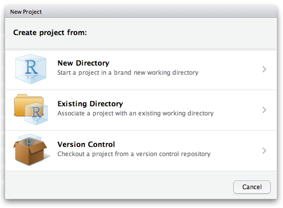
RStudio projects
- Feature for keeping all files associated with project together
- Our labs and exercises are each associated with a project
- Always start a new analysis by creating a new project. Keep all data and .qmd files associated with that project in your project folder.
- Open the project by double-clicking on your project file - R now knows that the folder containing your project file is the working directory.
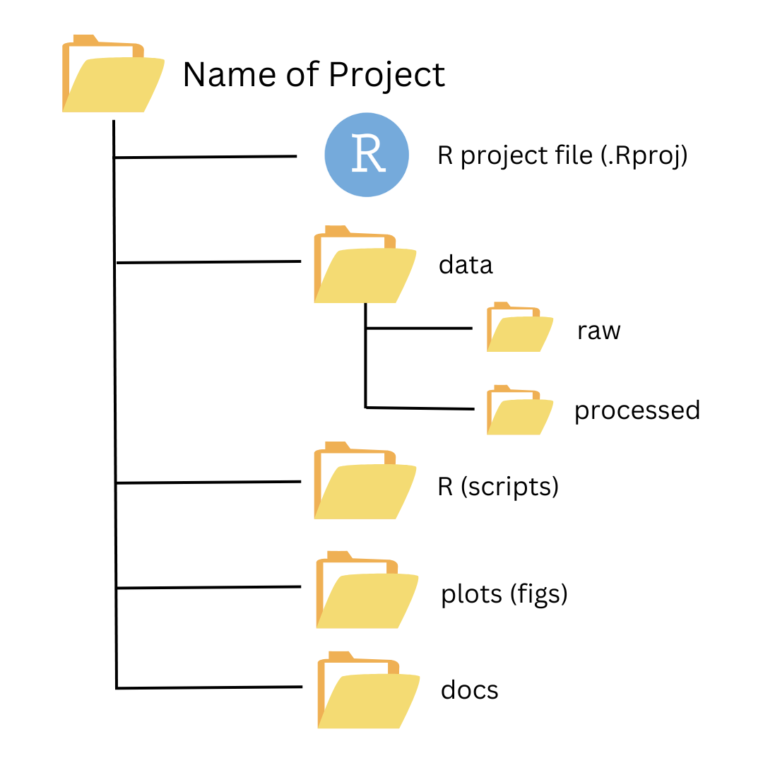
Project organization
- Save .Rproj file in main project folder
- Make folders for data, scripts (.qmd files), figures, and docs (reports, etc.)
Which type is x? Why?
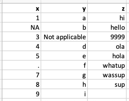
# A tibble: 9 × 3
  x     y              z
  <chr> <chr>          <chr>
1 1     a              hi
2 <NA>  b              hello
3 3     Not applicable 9999
4 4     d              ola
5 5     e              hola
6 .     f              whatup
7 7     g              wassup
8 8     h              sup
9 9 i <NA> Favorite foods
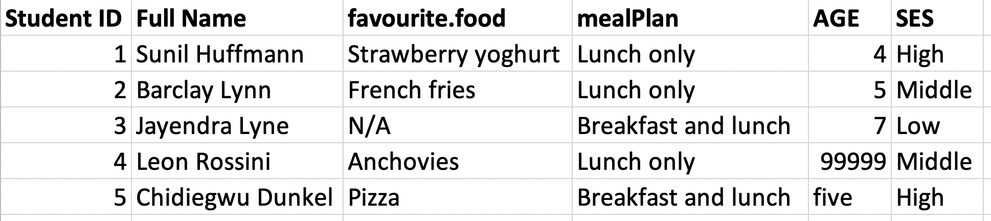
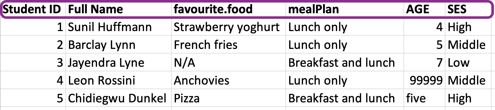
Variable names
Handling NAs
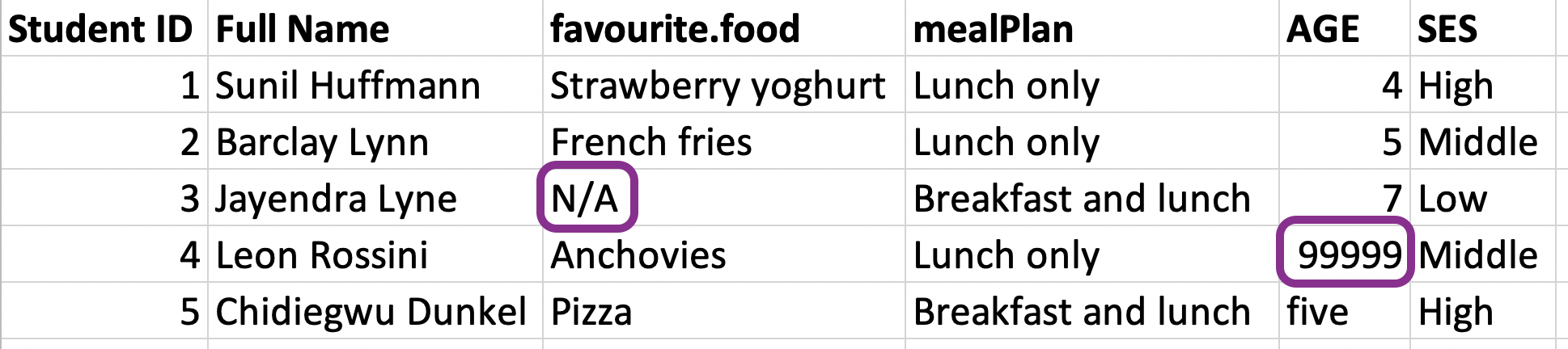
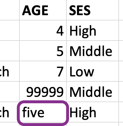
Make age numeric
fav_food <- fav_food |>
  mutate(
    age = if_else(age == "five", "5", age),
    age = as.numeric(age)
    )

fav_food
# A tibble: 5 × 6
student_id full_name favourite_food meal_plan age ses
<dbl> <chr> <chr> <chr> <dbl> <chr>
1 1 Sunil Huffmann Strawberry yoghurt Lunch only 4 High
2 2 Barclay Lynn French fries Lunch only 5 Midd…
3 3 Jayendra Lyne <NA> Breakfast and lunch 7 Low
4 4 Leon Rossini Anchovies Lunch only NA Midd…
5 5 Chidiegwu Dunkel Pizza Breakfast and lunch 5 High