Recoding data

Environmental Data Analysis and Visualization

https://mrne222-sp25.github.io/website/

There are a LOT of different ways to recode and transform your data in R.

We will cover a few of them, but Google is your friend to figure out how to recode in your own unique use cases.

Code-along: recoding functions

Code-along using the `iris` dataset

First load packages:

library(tidyverse)
library(janitor)

Clean the data names (iris is a built-in dataset that comes with R)

iris <- as_tibble(iris) |>
  clean_names()

iris

# A tibble: 150 × 5
   sepal_length sepal_width petal_length petal_width species
          <dbl>       <dbl>        <dbl>       <dbl> <fct>  
 1          5.1         3.5          1.4         0.2 setosa 
 2          4.9         3            1.4         0.2 setosa 
 3          4.7         3.2          1.3         0.2 setosa 
 4          4.6         3.1          1.5         0.2 setosa 
 5          5           3.6          1.4         0.2 setosa 
 6          5.4         3.9          1.7         0.4 setosa 
 7          4.6         3.4          1.4         0.3 setosa 
 8          5           3.4          1.5         0.2 setosa 
 9          4.4         2.9          1.4         0.2 setosa 
10          4.9         3.1          1.5         0.1 setosa 
# ℹ 140 more rows

Recode species so that setosa = “a”, versicolor = “b”, and virginica = “c”

distinct(iris, species)

# A tibble: 3 × 1
  species   
  <fct>     
1 setosa    
2 versicolor
3 virginica

iris |>
  mutate(species = case_match(species, "setosa" ~ "a", 
                              "versicolor" ~ "b", 
                              "virginica" ~ "c")) |> 
  distinct(species)

# A tibble: 3 × 1
  species
  <chr>  
1 a      
2 b      
3 c

Use .default argument if you want to keep some values the same

iris |>
  mutate(species = case_match(species, "setosa" ~ "a",
                              .default = species)) |> 
  distinct(species)

# A tibble: 3 × 1
  species   
  <chr>     
1 a         
2 versicolor
3 virginica

Use `mutate()` and `if_else()` to replace values based on certain conditions

If petal_length is less than three, recode petal_length to “short”. Otherwise (“else”) recode petal_length to “long”.

iris

# A tibble: 150 × 5
   sepal_length sepal_width petal_length petal_width species
          <dbl>       <dbl>        <dbl>       <dbl> <fct>  
 1          5.1         3.5          1.4         0.2 setosa 
 2          4.9         3            1.4         0.2 setosa 
 3          4.7         3.2          1.3         0.2 setosa 
 4          4.6         3.1          1.5         0.2 setosa 
 5          5           3.6          1.4         0.2 setosa 
 6          5.4         3.9          1.7         0.4 setosa 
 7          4.6         3.4          1.4         0.3 setosa 
 8          5           3.4          1.5         0.2 setosa 
 9          4.4         2.9          1.4         0.2 setosa 
10          4.9         3.1          1.5         0.1 setosa 
# ℹ 140 more rows

Use `mutate()` and `if_else()` to replace values based on certain conditions

If petal_length is less than three, recode petal_length to “short”. Otherwise (“else”) recode petal_length to “long”.

iris |>
  mutate(petal_length = if_else(petal_length < 3, "short", "long"))

# A tibble: 150 × 5
   sepal_length sepal_width petal_length petal_width species
          <dbl>       <dbl> <chr>              <dbl> <fct>  
 1          5.1         3.5 short                0.2 setosa 
 2          4.9         3   short                0.2 setosa 
 3          4.7         3.2 short                0.2 setosa 
 4          4.6         3.1 short                0.2 setosa 
 5          5           3.6 short                0.2 setosa 
 6          5.4         3.9 short                0.4 setosa 
 7          4.6         3.4 short                0.3 setosa 
 8          5           3.4 short                0.2 setosa 
 9          4.4         2.9 short                0.2 setosa 
10          4.9         3.1 short                0.1 setosa 
# ℹ 140 more rows

Create a new variable if you want to preserve the original values

iris |>
  mutate(petal_category = if_else(petal_length < 3, "short", "long"))

# A tibble: 150 × 6
   sepal_length sepal_width petal_length petal_width species petal_category
          <dbl>       <dbl>        <dbl>       <dbl> <fct>   <chr>         
 1          5.1         3.5          1.4         0.2 setosa  short         
 2          4.9         3            1.4         0.2 setosa  short         
 3          4.7         3.2          1.3         0.2 setosa  short         
 4          4.6         3.1          1.5         0.2 setosa  short         
 5          5           3.6          1.4         0.2 setosa  short         
 6          5.4         3.9          1.7         0.4 setosa  short         
 7          4.6         3.4          1.4         0.3 setosa  short         
 8          5           3.4          1.5         0.2 setosa  short         
 9          4.4         2.9          1.4         0.2 setosa  short         
10          4.9         3.1          1.5         0.1 setosa  short         
# ℹ 140 more rows

Use `case_when()` for more complicated conditional statements

If petal_length is less than or equal to 2, recode petal_length to “small”. If petal_length is greater than 2 and less than or equal to 5, recode to “medium”. If petal_length is greater than 5, recode to “large”.

iris |>
  mutate(petal_category = case_when(petal_length <= 2 ~ "small", 
                                    petal_length > 2 & sepal_length <= 5 ~ "medium", 
                                    petal_length > 5 ~ "large")) |> 
  distinct(petal_category)

# A tibble: 4 × 1
  petal_category
  <chr>         
1 small         
2 <NA>          
3 medium        
4 large

Use `TRUE` to index values that were not already defined

For all other values of petal_length, recode to “other”.

iris |>
  mutate(petal_category = case_when(petal_length <= 2 ~ "small", 
                                    petal_length > 2 & sepal_length <= 5 ~ "medium", 
                                    petal_length > 5 ~ "large",
                                    TRUE ~ "other")) |> 
  distinct(petal_category)

# A tibble: 4 × 1
  petal_category
  <chr>         
1 small         
2 other         
3 medium        
4 large

An example, with some data wrangling too

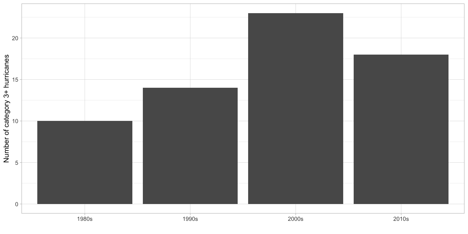
Calculate number of category 3, 4, and 5 storms each decade and plot the results.

The data:

storms |>
  select(name, year, month, day, hour, category)

# A tibble: 19,537 × 6
   name   year month   day  hour category
   <chr> <dbl> <dbl> <int> <dbl>    <dbl>
 1 Amy    1975     6    27     0       NA
 2 Amy    1975     6    27     6       NA
 3 Amy    1975     6    27    12       NA
 4 Amy    1975     6    27    18       NA
 5 Amy    1975     6    28     0       NA
 6 Amy    1975     6    28     6       NA
 7 Amy    1975     6    28    12       NA
 8 Amy    1975     6    28    18       NA
 9 Amy    1975     6    29     0       NA
10 Amy    1975     6    29     6       NA
# ℹ 19,527 more rows

The process:

filter to remove years from decades that have incomplete data
filter so storm category is greater than or equal to 3
create new variable (decade)
group by decade and use summarize to calculate total number of

We’ll need to create new categorical variable (decade), then group and summarize by that variable.

storms |>
  select(name, year, month, day, hour, category)

# A tibble: 19,537 × 6
   name   year month   day  hour category
   <chr> <dbl> <dbl> <int> <dbl>    <dbl>
 1 Amy    1975     6    27     0       NA
 2 Amy    1975     6    27     6       NA
 3 Amy    1975     6    27    12       NA
 4 Amy    1975     6    27    18       NA
 5 Amy    1975     6    28     0       NA
 6 Amy    1975     6    28     6       NA
 7 Amy    1975     6    28    12       NA
 8 Amy    1975     6    28    18       NA
 9 Amy    1975     6    29     0       NA
10 Amy    1975     6    29     6       NA
# ℹ 19,527 more rows

First filter so year is between 1980 and 2020 and category >= 3

We need to remove years from decades where data is incomplete.

storms |>
  select(name, year, month, day, hour, category) |> 
  filter(year >= 1980, 
         year < 2020, 
         category >= 3)

# A tibble: 1,090 × 6
   name   year month   day  hour category
   <chr> <dbl> <dbl> <int> <dbl>    <dbl>
 1 Allen  1980     8     4     0        3
 2 Allen  1980     8     4     6        4
 3 Allen  1980     8     4    12        4
 4 Allen  1980     8     4    18        4
 5 Allen  1980     8     5     0        5
 6 Allen  1980     8     5     6        5
 7 Allen  1980     8     5    12        5
 8 Allen  1980     8     5    18        5
 9 Allen  1980     8     6     0        5
10 Allen  1980     8     6     6        4
# ℹ 1,080 more rows

Next group by year and storm name and calculate the max category reached for each storm and year

Code
Output

storms |>
  select(name, year, month, day, hour, category) |> 
  filter(year >= 1980, 
         year < 2020, 
         category > 3) |>
  group_by(name, year) |> 
  summarize(maxcat = max(category))

# A tibble: 65 × 3
# Groups:   name [63]
   name       year maxcat
   <chr>     <dbl>  <dbl>
 1 Allen      1980      5
 2 Andrew     1992      5
 3 Bill       2009      4
 4 Bret       1999      4
 5 Charley    2004      4
 6 Cindy      1999      4
 7 Claudette  1991      4
 8 Danielle   2010      4
 9 Dean       2007      5
10 Debby      1982      4
# ℹ 55 more rows

Next, create a `decade` variable using `mutate()` and `case_when()` based on the `year` variable

Code
Output

storms |>
  select(name, year, month, day, hour, category) |>
  filter(year >= 1980, 
         year < 2020, 
         category > 3) |>
  group_by(name, year) |>
  summarize(maxcat = max(category)) |>
  mutate(decade = case_when(year %in% 1980:1989 ~ "1980s", 
                            year %in% 1990:1999 ~ "1990s",
                            year %in% 2000:2009 ~ "2000s", 
                            year %in% 2010:2019 ~ "2010s"))

# A tibble: 65 × 4
# Groups:   name [63]
   name       year maxcat decade
   <chr>     <dbl>  <dbl> <chr> 
 1 Allen      1980      5 1980s 
 2 Andrew     1992      5 1990s 
 3 Bill       2009      4 2000s 
 4 Bret       1999      4 1990s 
 5 Charley    2004      4 2000s 
 6 Cindy      1999      4 1990s 
 7 Claudette  1991      4 1990s 
 8 Danielle   2010      4 2010s 
 9 Dean       2007      5 2000s 
10 Debby      1982      4 1980s 
# ℹ 55 more rows

Finally, group by the new decade variable and count the number of storms in each decade

Code
Output

storms |>
  select(name, year, month, day, hour, category) |> 
  filter(year >= 1980, 
         year < 2020, 
         category > 3) |>
  group_by(name, year) |>
  summarize(maxcat = max(category)) |>
  mutate(decade = case_when(year %in% 1980:1989 ~ "1980s",
                            year %in% 1990:1999 ~ "1990s",
                            year %in% 2000:2009 ~ "2000s",
                            year %in% 2010:2019 ~ "2010s")) |>
  group_by(decade) |> 
  summarize(n = n())

# A tibble: 4 × 2
  decade     n
  <chr>  <int>
1 1980s     10
2 1990s     14
3 2000s     23
4 2010s     18

storms |>
  filter(year >= 1980,
         year < 2020,
         category > 3) |>
  group_by(name, year) |>
  summarize(maxcat = max(category)) |>
  mutate(decade = case_when(year %in% 1980:1989 ~ "1980s",
                            year %in% 1990:1999 ~ "1990s",
                            year %in% 2000:2009 ~ "2000s",
                            year %in% 2010:2019 ~ "2010s")) |>
  group_by(decade) |>
  summarize(n = n()) |>
  ggplot(aes(x = decade, y = n)) + 
  geom_bar(stat = "identity") + 
  labs(x = "", y = "Number of category 3+ hurricanes") + 
  theme_light()

Recoding data

There are a LOT of different ways to recode and transform your data in R.

Code-along: recoding functions

Code-along using the iris dataset

Recode species so that setosa = “a”, versicolor = “b”, and virginica = “c”

Use .default argument if you want to keep some values the same

Use mutate() and if_else() to replace values based on certain conditions

Use mutate() and if_else() to replace values based on certain conditions

Create a new variable if you want to preserve the original values

Use case_when() for more complicated conditional statements

Use TRUE to index values that were not already defined

An example, with some data wrangling too

Calculate number of category 3, 4, and 5 storms each decade and plot the results.

First filter so year is between 1980 and 2020 and category >= 3

Next group by year and storm name and calculate the max category reached for each storm and year

Next, create a decade variable using mutate() and case_when() based on the year variable

Finally, group by the new decade variable and count the number of storms in each decade

and then plot!

Code-along using the `iris` dataset

Use `mutate()` and `if_else()` to replace values based on certain conditions

Use `mutate()` and `if_else()` to replace values based on certain conditions

Use `case_when()` for more complicated conditional statements

Use `TRUE` to index values that were not already defined

Next, create a `decade` variable using `mutate()` and `case_when()` based on the `year` variable