Doing data science

Environmental Data Analysis and Visualization

What’s in a data analysis?

Five core activities of data analysis

Stating and refining the question
Exploring the data
Building formal statistical models
Interpreting the results
Communicating the results

Roger D. Peng and Elizabeth Matsui. “The Art of Data Science.” A Guide for Anyone Who Works with Data. Skybrude Consulting, LLC (2015).

Stating and refining the question

Six types of questions

Descriptive: summarize a characteristic of a set of data
Exploratory: analyze to see if there are patterns, trends, or relationships between variables (hypothesis generating)
Inferential: analyze patterns, trends, or relationships in representative data from a population
Predictive: make predictions for individuals or groups of individuals
Causal: whether changing one factor will change another factor, on average, in a population
Mechanistic: explore “how” as opposed to whether

Jeffery T. Leek and Roger D. Peng. “What is the question?.” Science 347.6228 (2015): 1314-1315.

Ex: COVID-19 and Vitamin D

Descriptive: frequency of hospitalizations due to COVID-19 in a data set collected from a group of individuals
Exploratory: examine relationships between a range of dietary factors and COVID-19 hospitalizations
Inferential: examine whether any relationships between taking Vitamin D supplements and COVID-19 hospitalizations found in the sample hold for the population at large
Predictive: predict what types of people will take Vitamin D supplements during the next year
Causal: test whether the hospitalization rate differs for people with COVID-19 who were randomly assigned to take Vitamin D supplements vs. those who were not assigned to take Vitamin D
Mechanistic: investigate the physiological mechanism by which increased vitamin D intake leads to a reduction in the number of viral illnesses

Questions to ask when begining an analysis

Do you have appropriate data to answer your question?
Do you have information on confounding variables (other variables that can affect the variable(s) of interest)?
Was the data you’re working with collected in a way that introduces bias?

Beware of confounding variables

Suppose I collect data on sunburns and ice cream consumption and find that higher ice cream consumption is associated with a higher probability of sunburn.

Does that mean that ice cream consumption causes sunburn?
What might be a confounding variable?
Can you think of an example from ecology/the environment?
How can we control for confounding variables in our analyses?

Beware of biased data

Suppose I want to estimate the average number of children in households in St. Mary’s County. I conduct a survey at an elementary school in the county and ask students at this elementary school how many children, including themselves, live in their house. Then, I take the average of the responses.

Is this a biased or an unbiased estimate of the number of children in households in the county?
If biased, will the value be an overestimate or underestimate?
How can we minimze bias in our analyses?

Exploratory data analysis

Exploratory data analysis checklist

Formulate your question
Read in your data
Check the dimensions
Look at the top and the bottom of your data
Validate with at least one external data source
Make a plot
Try the easy solution first

Formulate your question

Consider scope:

Are air pollution levels higher on the east coast than on the west coast?
Are hourly ozone levels on average higher in New York City than they are in Los Angeles?
Do counties in the eastern United States have higher ozone levels than counties in the western United States?
Most importantly: “Do I have the right data to answer this question?”

Read in your data

Place your data in a folder called data
Read it into R with read_csv() or friends (read_delim(), read_excel(), etc.)

library(readxl)
fav_food <- read_excel("data/favourite-food.xlsx")
fav_food

# A tibble: 5 × 6
  `Student ID` `Full Name`      favourite.food     mealPlan          AGE   SES  
         <dbl> <chr>            <chr>              <chr>             <chr> <chr>
1            1 Sunil Huffmann   Strawberry yoghurt Lunch only        4     High 
2            2 Barclay Lynn     French fries       Lunch only        5     Midd…
3            3 Jayendra Lyne    N/A                Breakfast and lu… 7     Low  
4            4 Leon Rossini     Anchovies          Lunch only        99999 Midd…
5            5 Chidiegwu Dunkel Pizza              Breakfast and lu… five  High

`clean_names()`

If the variable names are not formatted in snake_case, use janitor::clean_names()

library(janitor)
fav_food %>% clean_names()

# A tibble: 5 × 6
  student_id full_name        favourite_food     meal_plan           age   ses  
       <dbl> <chr>            <chr>              <chr>               <chr> <chr>
1          1 Sunil Huffmann   Strawberry yoghurt Lunch only          4     High 
2          2 Barclay Lynn     French fries       Lunch only          5     Midd…
3          3 Jayendra Lyne    N/A                Breakfast and lunch 7     Low  
4          4 Leon Rossini     Anchovies          Lunch only          99999 Midd…
5          5 Chidiegwu Dunkel Pizza              Breakfast and lunch five  High

Case study: NYC Squirrels!

The Squirrel Census is a multimedia science, design, and storytelling project focusing on the Eastern gray (Sciurus carolinensis). They count squirrels and present their findings to the public.
This table contains squirrel data for each of the 3,023 sightings, including location coordinates, age, primary and secondary fur color, elevation, activities, communications, and interactions between squirrels and with humans.

# devtools::install_github("mine-cetinkaya-rundel/nycsquirrels18")
library(nycsquirrels18)

Look at dataset info

?squirrels

Check the dimensions

dim(squirrels)

[1] 3023   35

Look at the top…

squirrels |>
  head()

# A tibble: 6 × 35
   long   lat unique_squirrel_id hectare shift date       hectare_squirrel_num…¹
  <dbl> <dbl> <chr>              <chr>   <chr> <date>                      <dbl>
1 -74.0  40.8 13A-PM-1014-04     13A     PM    2018-10-14                      4
2 -74.0  40.8 15F-PM-1010-06     15F     PM    2018-10-10                      6
3 -74.0  40.8 19C-PM-1018-02     19C     PM    2018-10-18                      2
4 -74.0  40.8 21B-AM-1019-04     21B     AM    2018-10-19                      4
5 -74.0  40.8 23A-AM-1018-02     23A     AM    2018-10-18                      2
6 -74.0  40.8 38H-PM-1012-01     38H     PM    2018-10-12                      1
# ℹ abbreviated name: ¹hectare_squirrel_number
# ℹ 28 more variables: age <chr>, primary_fur_color <chr>,
#   highlight_fur_color <chr>,
#   combination_of_primary_and_highlight_color <chr>, color_notes <chr>,
#   location <chr>, above_ground_sighter_measurement <chr>,
#   specific_location <chr>, running <lgl>, chasing <lgl>, climbing <lgl>,
#   eating <lgl>, foraging <lgl>, other_activities <chr>, kuks <lgl>, …

…and the bottom

squirrels |> 
  tail()

# A tibble: 6 × 35
   long   lat unique_squirrel_id hectare shift date       hectare_squirrel_num…¹
  <dbl> <dbl> <chr>              <chr>   <chr> <date>                      <dbl>
1 -74.0  40.8 6D-PM-1020-01      06D     PM    2018-10-20                      1
2 -74.0  40.8 21H-PM-1018-01     21H     PM    2018-10-18                      1
3 -74.0  40.8 31D-PM-1006-02     31D     PM    2018-10-06                      2
4 -74.0  40.8 37B-AM-1018-04     37B     AM    2018-10-18                      4
5 -74.0  40.8 21C-PM-1006-01     21C     PM    2018-10-06                      1
6 -74.0  40.8 7G-PM-1018-04      07G     PM    2018-10-18                      4
# ℹ abbreviated name: ¹hectare_squirrel_number
# ℹ 28 more variables: age <chr>, primary_fur_color <chr>,
#   highlight_fur_color <chr>,
#   combination_of_primary_and_highlight_color <chr>, color_notes <chr>,
#   location <chr>, above_ground_sighter_measurement <chr>,
#   specific_location <chr>, running <lgl>, chasing <lgl>, climbing <lgl>,
#   eating <lgl>, foraging <lgl>, other_activities <chr>, kuks <lgl>, …

Validate with at least one external data source

squirrels %>%
  select(long, lat) %>%
  print(n = 15)

# A tibble: 3,023 × 2
    long   lat
   <dbl> <dbl>
 1 -74.0  40.8
 2 -74.0  40.8
 3 -74.0  40.8
 4 -74.0  40.8
 5 -74.0  40.8
 6 -74.0  40.8
 7 -74.0  40.8
 8 -74.0  40.8
 9 -74.0  40.8
10 -74.0  40.8
11 -74.0  40.8
12 -74.0  40.8
13 -74.0  40.8
14 -74.0  40.8
15 -74.0  40.8
# ℹ 3,008 more rows

Make a plot

ggplot(squirrels, aes(x = long, y = lat)) +
  geom_point(alpha = 0.2)

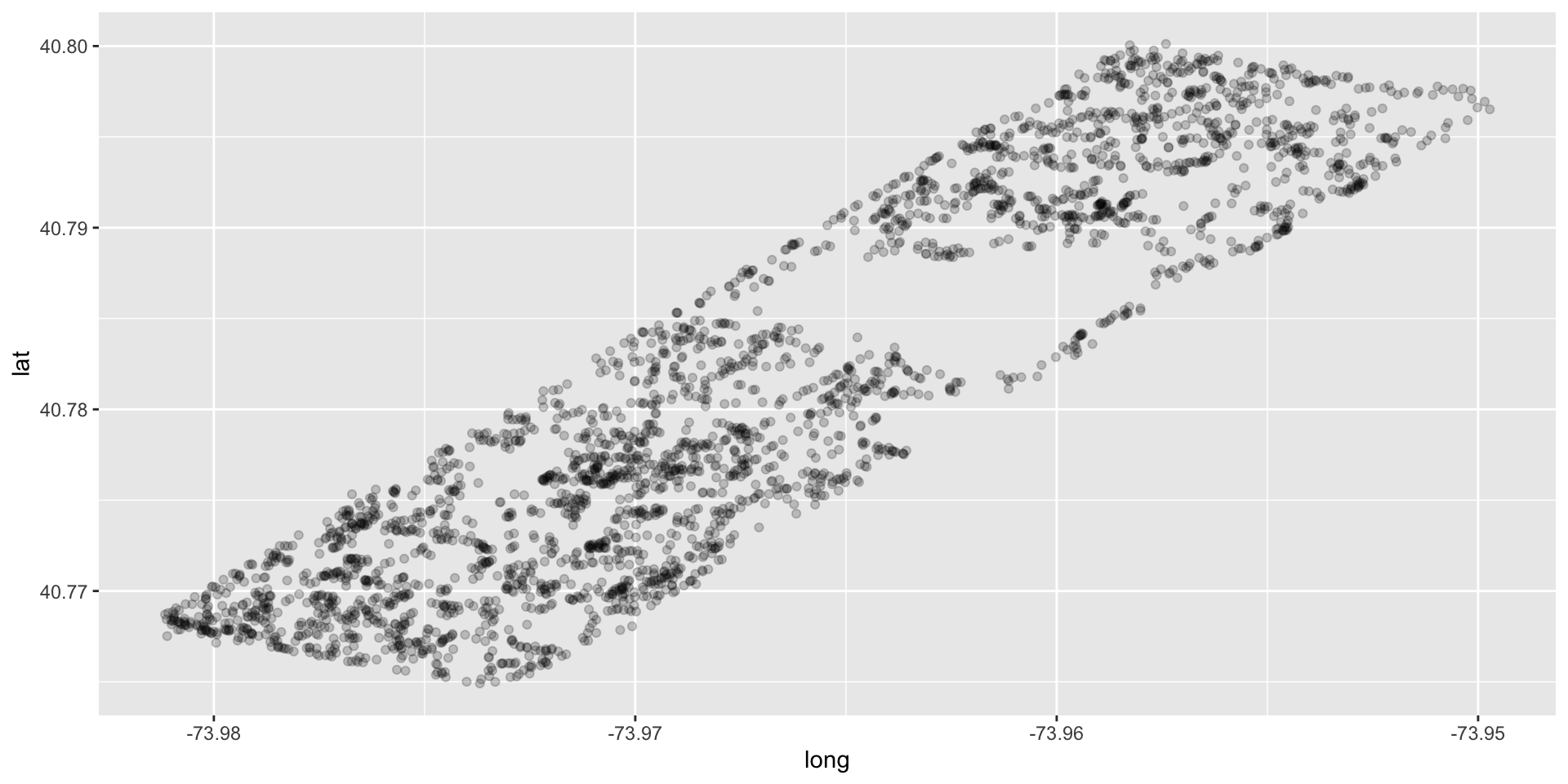
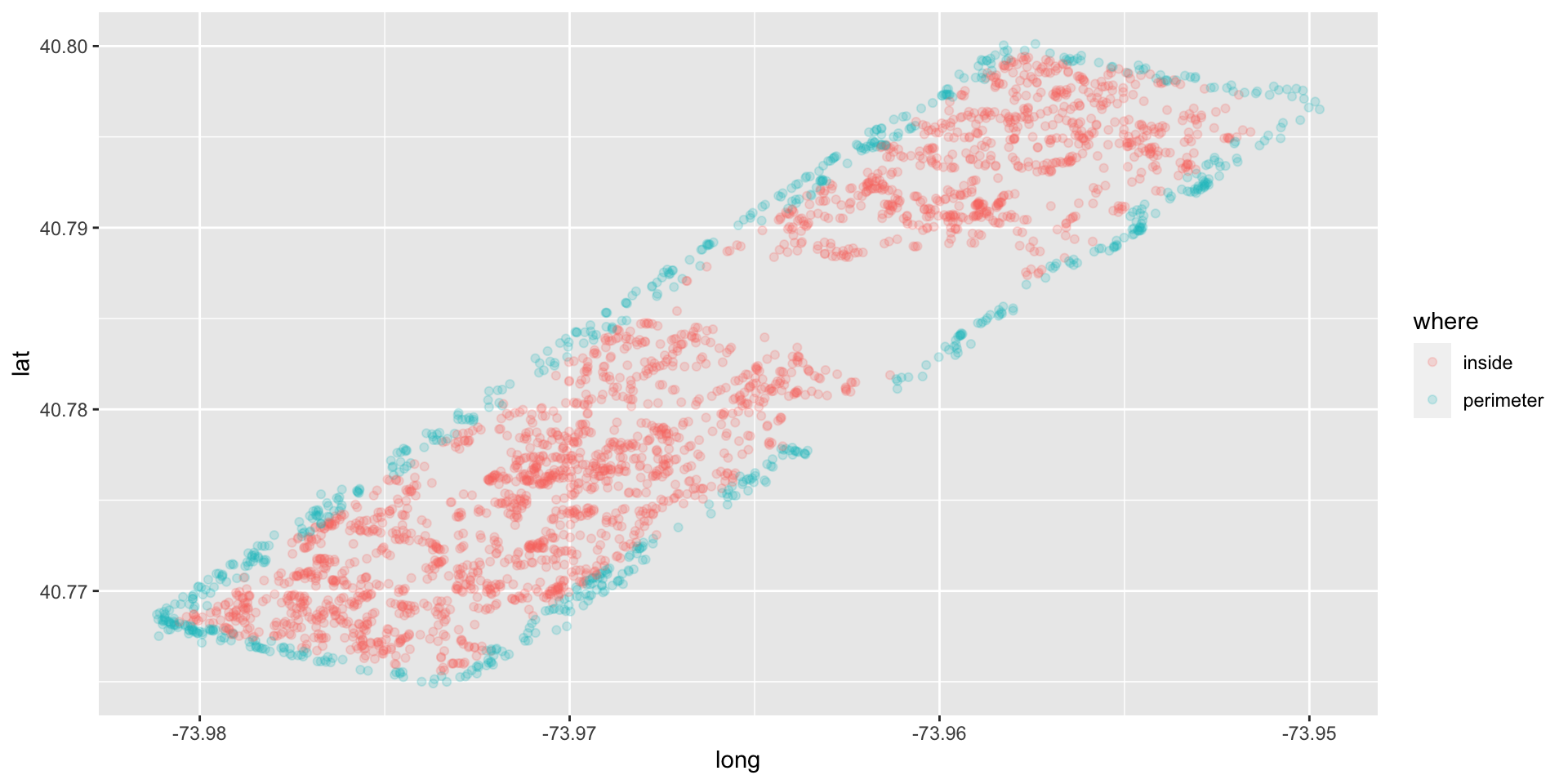
Hypothesis: There will be a higher density of sightings on the perimeter than inside the park.

squirrels <- squirrels %>%
  separate(hectare, into = c("NS", "EW"), sep = 2, remove = FALSE) %>%
  mutate(where = if_else(NS %in% c("01", "42") | EW %in% c("A", "I"), "perimeter", "inside")) 

ggplot(squirrels, aes(x = long, y = lat, color = where)) +
  geom_point(alpha = 0.2)

Then go deeper…

Plot
Code

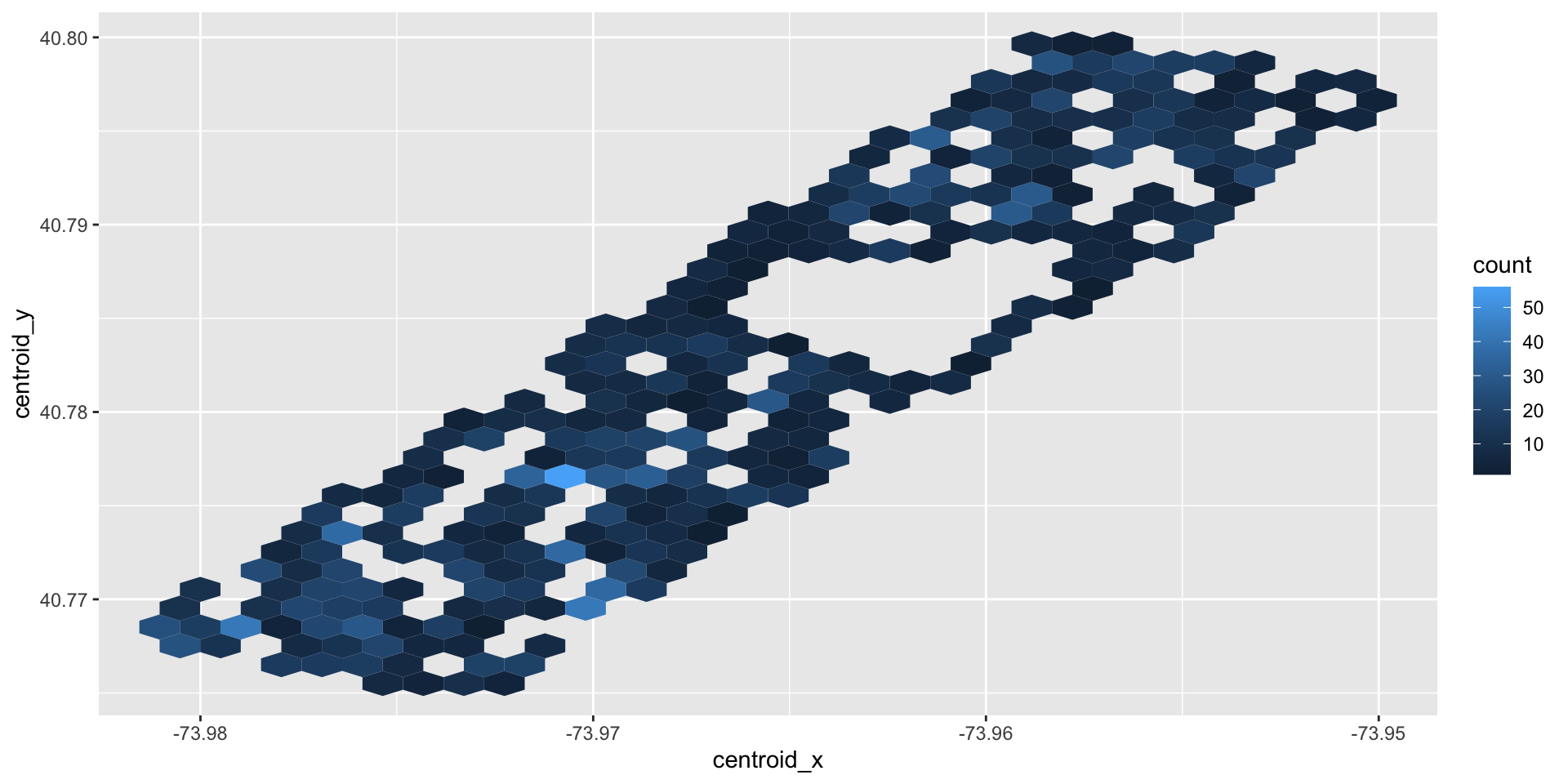
hectare_counts <- squirrels %>%
  group_by(hectare) %>%
  summarise(n = n()) 

hectare_centroids <- squirrels %>%
  group_by(hectare) %>%
  summarise(
    centroid_x = mean(long),
    centroid_y = mean(lat)
  )

squirrels %>%
  left_join(hectare_counts, by = "hectare") %>%
  left_join(hectare_centroids, by = "hectare") %>%
  ggplot(aes(x = centroid_x, y = centroid_y, color = n)) +
  geom_hex()

Communicating for your audience

Avoid: Jargon, uninterpreted results, lengthy output
Pay attention to: Organization, presentation, flow
Don’t forget about: Code style, coding best practices, meaningful commits
Be open to: Suggestions, feedback, taking (calculated) risks