Functions: The details

Environmental Data Analysis and Visualization

Recall, to turn your code into a function you need three things:

A name
The arguments
The body

Mutate functions

Functions that work well inside of mutate() and filter() because they return output that is the same length as the input.

An example: calculate z-score

Z-scores rescale a vector to have a mean of zero and a standard deviation of one. It can be useful when you want to do stats on datasets with very different value ranges.

x <- c(0.01, 0.05, 0.004)

y <- c(40402, 495993, 589290)

(x - mean(x, na.rm = TRUE)) / sd(x, na.rm = TRUE)

[1] -0.4532125  1.1463610 -0.6931485

(y - mean(x, na.rm = TRUE)) / sd(y, na.rm = TRUE)

[1] 0.1375637 1.6887948 2.0064595

An example: calculate z-score

Turn it into a function:

zscore <- function(x){
  (x - mean(x, na.rm = TRUE)) / sd(x, na.rm = TRUE)
}

zscore(x)

[1] -0.4532125  1.1463610 -0.6931485

zscore(y)

[1] -1.1400423  0.4111888  0.7288535

An example: recode values in a vector

Create a function called clamp() that recodes values in a vector to be equal to some user-supplied minimum or maximum value if they are less than or greater than the min/max.

Have:

 [1]  1  2  3  4  5  6  7  8  9 10

Want:

 [1] 3 3 3 4 5 6 7 7 7 7

An example: recode values in a vector

Create a function called clamp() that recodes values in a vector to be equal to some user-supplied minimum or maximum value if they are less than or greater than the min/max.

Define the function:

clamp <- function(x, min, max) {
  case_when(
    x < min ~ min,
    x > max ~ max,
    TRUE ~ x
  )
}

Execute the function:

clamp(1:10, min = 3, max = 7)

 [1] 3 3 3 4 5 6 7 7 7 7

An example: mutate function with character data

Make the first letter of each value upper case.

Have:

[1] "hello"   "goodbye" "see ya"

Want:

[1] "Hello"   "Goodbye" "See ya"

An example: mutate function with character data

This one’s a bit more complicated. First work out the code outside of the function.

Ultimately, we can use the str_sub() function to sub out the lower case letter with an upper case letter.

From the help file:

str_sub(string, start = 1L, end = -1L, omit_na = FALSE) <- value

word <- "hello"
word

[1] "hello"

str_sub(word, 1, 1) <- "H"
word

[1] "Hello"

An example: mutate function with character data

We can use the str_sub() and str_to_upper() functions to programatically determine the replacement value.

word <- "hello"
word

[1] "hello"

str_to_upper(str_sub(word, 1, 1))

[1] "H"

An example: mutate function with character data

Now put it all together.

word

[1] "hello"

str_sub(word, 1, 1) <- str_to_upper(str_sub(word, 1, 1))
word

[1] "Hello"

An example: mutate function with character data

It worked. NOW make it a function.

Define the function:

first_upper <- function(x) {
  str_sub(x, 1, 1) <- str_to_upper(str_sub(x, 1, 1))
  x
}

Execute the function:

first_upper(word)

[1] "Hello"

string <- c("hello", "goodbye", "see ya")
first_upper(string)

[1] "Hello"   "Goodbye" "See ya"

Summary functions

Return a single value for use in summarize()

An example: calculate standard error

se = sd / \(n^{2}\)

se <- function(x){
  sd(x, na.rm = TRUE) / sqrt(length(x))
}

x <- c(3, 6, 9)

se(x)

[1] 1.732051

An example: standard error

data <- tibble(x = c(1, 3, 5),
               y = c(6, 8, 9))

data

# A tibble: 3 × 2
      x     y
  <dbl> <dbl>
1     1     6
2     3     8
3     5     9

data |> 
  summarize(mean_x = mean(x), 
            se_x = se(x),
            mean_y = mean(y),
            se_y = se(y))

# A tibble: 1 × 4
  mean_x  se_x mean_y  se_y
   <dbl> <dbl>  <dbl> <dbl>
1      3  1.15   7.67 0.882

Summary function with multiple vector inputs

Mean absolute percent error to compare model predictions with absolute values:

mape <- function(actual, predicted) {
  sum(abs((actual - predicted) / actual)) / length(actual)
}

Data frame functions

Take a data frame as the first argument, some extra arguments that say what to do with it, and return a data frame or a vector.
Useful if you find yourself using the same wrangling or plotting pipeline for different data or subsets of data.

Get to know tidy evaluation

Have:

diamonds

# A tibble: 53,940 × 10
   carat cut       color clarity depth table price     x     y     z
   <dbl> <ord>     <ord> <ord>   <dbl> <dbl> <int> <dbl> <dbl> <dbl>
 1  0.23 Ideal     E     SI2      61.5    55   326  3.95  3.98  2.43
 2  0.21 Premium   E     SI1      59.8    61   326  3.89  3.84  2.31
 3  0.23 Good      E     VS1      56.9    65   327  4.05  4.07  2.31
 4  0.29 Premium   I     VS2      62.4    58   334  4.2   4.23  2.63
 5  0.31 Good      J     SI2      63.3    58   335  4.34  4.35  2.75
 6  0.24 Very Good J     VVS2     62.8    57   336  3.94  3.96  2.48
 7  0.24 Very Good I     VVS1     62.3    57   336  3.95  3.98  2.47
 8  0.26 Very Good H     SI1      61.9    55   337  4.07  4.11  2.53
 9  0.22 Fair      E     VS2      65.1    61   337  3.87  3.78  2.49
10  0.23 Very Good H     VS1      59.4    61   338  4     4.05  2.39
# ℹ 53,930 more rows

Get to know tidy evaluation

Want: Calculate the mean of a variable (mean_var) based on a grouping variable (group_var) from a dataframe df.

grouped_mean <- function(df, group_var, mean_var) {
  df |> 
    group_by(group_var) |> 
    summarize(mean(mean_var))
}

Get to know tidy evaluation

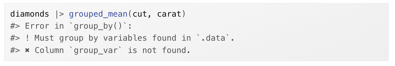
Why do we get an error?

Get to know tidy evaluation

Why do we get an error?

When function arguments indirectly refer to the name of a column, R takes it literally.

Get to know tidy evaluation

What we want to happen:

diamonds |> 
  group_by(cut) |> 
  summarize(mean(carat))

group by cut (or any other grouping variable)
calculate mean carat (or any other numeric variable)

What is actually happening:

diamonds |> 
  group_by(group_var) |> 
  summarize(mean(mean_var))

group_var and mean_var aren’t column names, they are the names of the arguments we defined in the grouped_mean() function.

Get to know tidy evaluation

Tidy evaluation allows us to refer to variable names directly when using tidyverse functions. However, special treatment is required when you use functions that use tidy evaluation.
{{}} are the special treatment we need to apply
How do you know which functions use tidy evaluation? You’ll know if you get an the error that your variable wasn’t found. You can also look in a function’s help file. Under Arguments, <tidy-select> or <data-masking> will be listed.

Proper data frame function with `{{}}`

Want: Calculate the mean of a variable (mean_var) based on a grouping variable (group_var) from the dataframe df.

grouped_mean <- function(df, group_var, mean_var) {
  df |> 
    group_by({{group_var}}) |> 
    summarize(mean({{mean_var}}))
}

The {{}} tells R to use the value you supplied for the grouped_var and mean_var arguments, not the literal argument names.

Proper data frame function with `{{}}`

Want: Calculate the mean of a variable (mean_var) based on a grouping variable (group_var) from the dataframe df.

diamonds |> 
  grouped_mean(cut, carat)

# A tibble: 5 × 2
  cut       `mean(carat)`
  <ord>             <dbl>
1 Fair              1.05 
2 Good              0.849
3 Very Good         0.806
4 Premium           0.892
5 Ideal             0.703

Plot functions

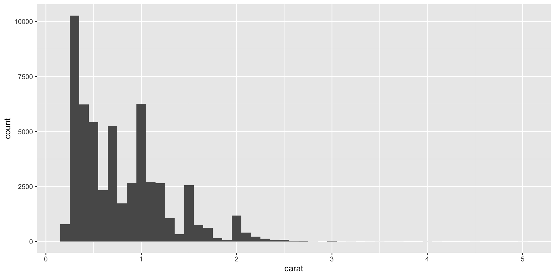
Want: I need to make a lot of histograms with different binwidths.

diamonds |> 
  ggplot(aes(x = carat)) +
  geom_histogram(binwidth = 0.5)

diamonds |> 
  ggplot(aes(x = carat)) +
  geom_histogram(binwidth = 0.05)

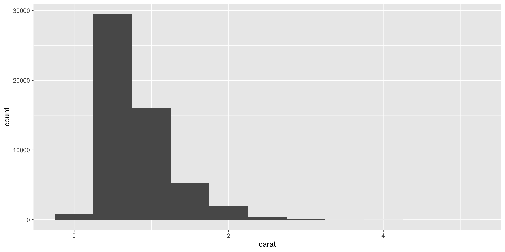
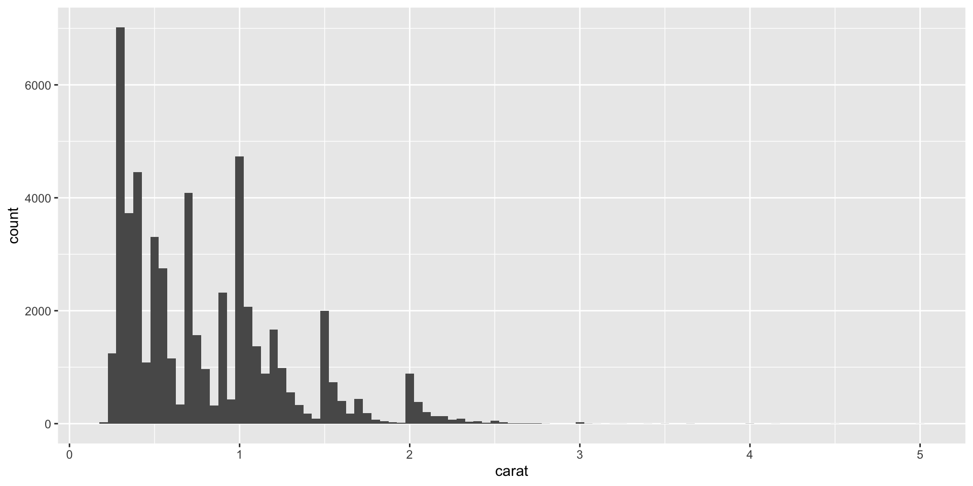
Make a plot function

Define the function. Put arguments that indirectly refer to column names in {{}}.

histogram <- function(df, var, binwidth){
  df |> 
    ggplot(aes(x = {{ var }})) +
    geom_histogram(binwidth = binwidth)
}

Use the function to make a plot.

diamonds |> 
  histogram(carat, 0.1)

Optional: Add components after running plot function

Our histogram() function returns a ggplot2 plot, meaning you can still add additional components if you want. Just remember to switch from |> to +:

diamonds |> 
  histogram(carat, 0.1) +
  labs(x = "Size (in carats)", y = "Number of diamonds")

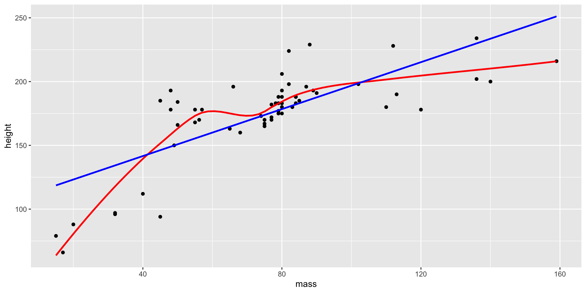
Plot function with more variables

Function to eyeball whether or not a dataset is linear by overlaying a smooth line and a straight line:

linearity_check <- function(df, x, y) {
  df |>
    ggplot(aes(x = {{ x }}, y = {{ y }})) +
    geom_point() +
    geom_smooth(method = "loess", formula = y ~ x, color = "red", se = FALSE) +
    geom_smooth(method = "lm", formula = y ~ x, color = "blue", se = FALSE) 
}

Run the function using the starwars dataset:

starwars |> 
  filter(mass < 1000) |> 
  linearity_check(mass, height)

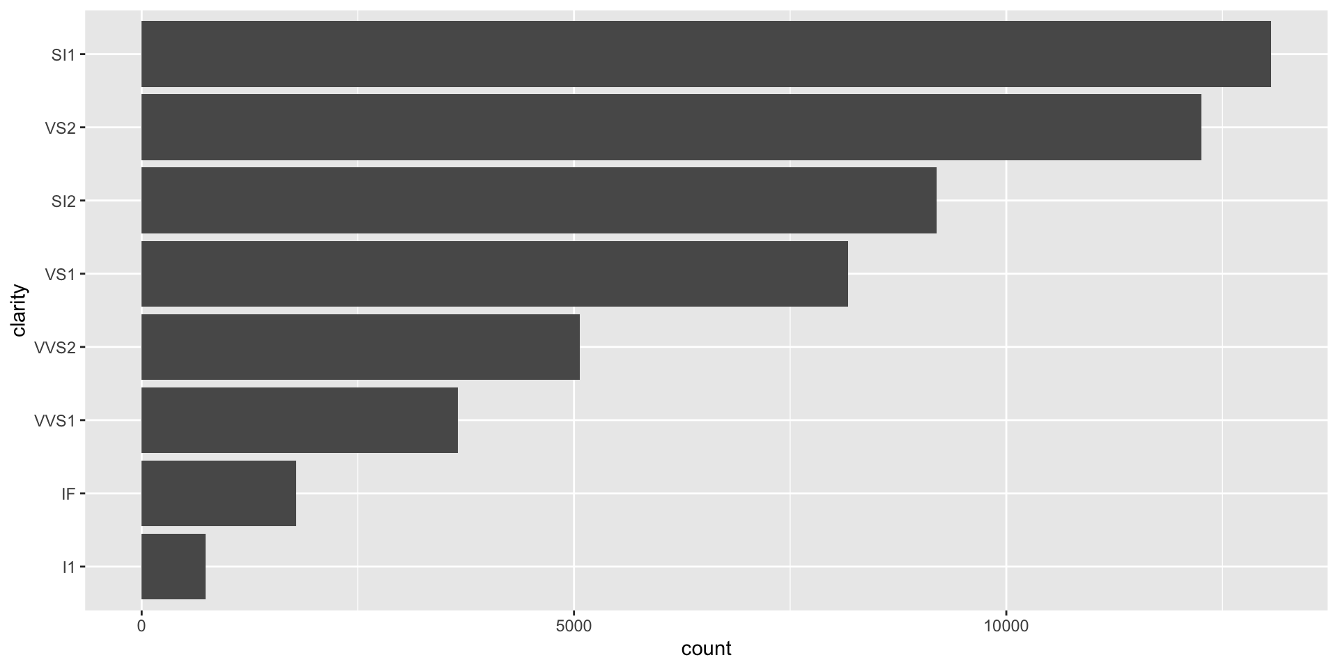
Make a function to wrangle then plot

Use the fct_infreq() function to sort factor levels according to frequency, then plot in a horizontal bar chart:

sorted_bars <- function(df, var) {
  df |> 
    mutate({{ var }} := fct_rev(fct_infreq({{ var }})))  |>
    ggplot(aes(y = {{ var }})) +
    geom_bar()
}

Use the function to wangle + plot:

diamonds |> 
  sorted_bars(clarity)

`:=` The “walrus operator”

You can only use = in a tidy function like mutate() when referring directly to a variable name:
mutate(new_variable = ...)
If you want to indirectly use a user-supplied variable name as an argument in your function, := let’s R know to look for the argument name supplied:
mutate({{var}} := ...)

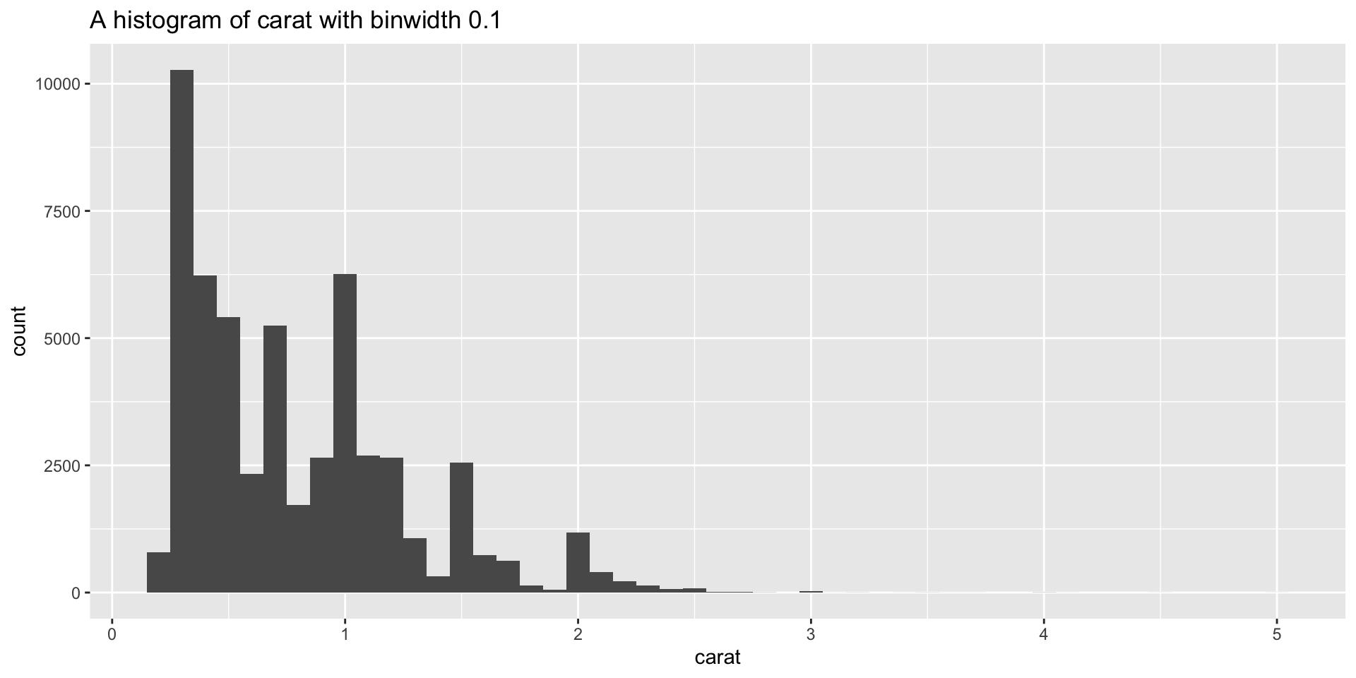
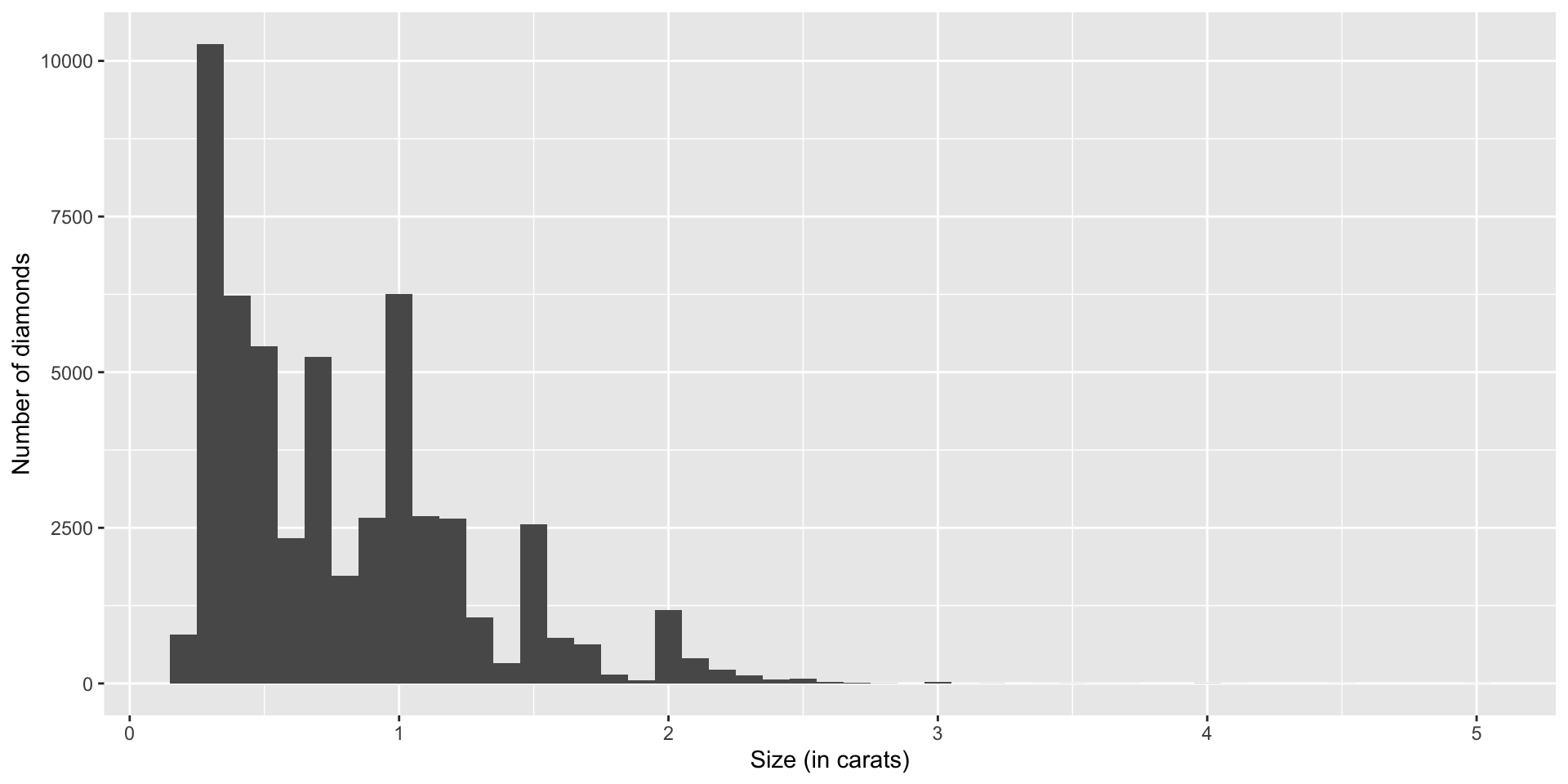
Label plots in a function based on user inputs

Add a plot title that labels the variable and binwidth:

histogram <- function(df, var, binwidth) {
  label <- rlang::englue("A histogram of {{var}} with binwidth {binwidth}")
  
  df |> 
    ggplot(aes(x = {{ var }})) + 
    geom_histogram(binwidth = binwidth) + 
    labs(title = label)
}

Make a plot:

diamonds |> histogram(carat, 0.1)

Functions: The details

Recall, to turn your code into a function you need three things:

Mutate functions

Mutate functions

An example: calculate z-score

An example: calculate z-score

An example: recode values in a vector

An example: recode values in a vector

An example: mutate function with character data

An example: mutate function with character data

An example: mutate function with character data

An example: mutate function with character data

An example: mutate function with character data

Summary functions

Summary functions

An example: calculate standard error

An example: standard error

Summary function with multiple vector inputs

Data frame functions

Data frame functions

Get to know tidy evaluation

Get to know tidy evaluation

Get to know tidy evaluation

Get to know tidy evaluation

Get to know tidy evaluation

Get to know tidy evaluation

Proper data frame function with {{}}

Proper data frame function with {{}}

Plot functions

Plot functions

Make a plot function

Optional: Add components after running plot function

Plot function with more variables

Make a function to wrangle then plot

:= The “walrus operator”

Label plots in a function based on user inputs

Proper data frame function with `{{}}`

Proper data frame function with `{{}}`

`:=` The “walrus operator”