More iteration use cases that can come in handy
ENST/MRNE 222 Environmental Data Analysis and Visualization
purrr::map() function
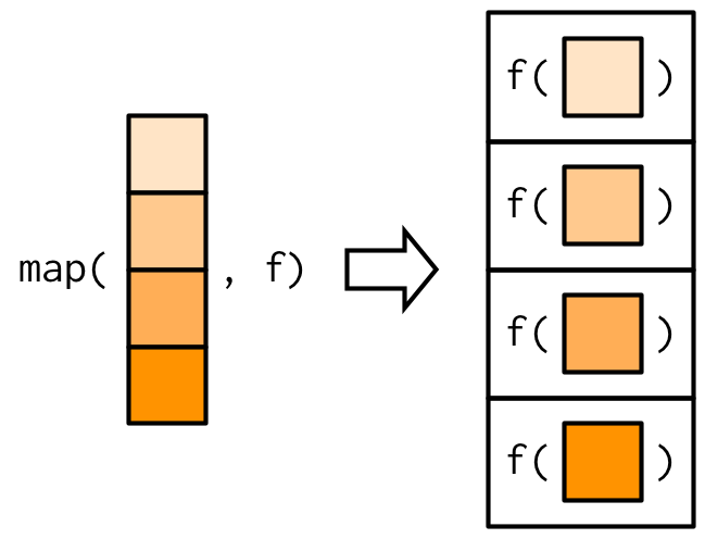
map()executes a function (.f) for each element of your input data (.x)- A list is always returned -
- Since the first argument is always the data (
.x),map()functions work well with piping (|>)
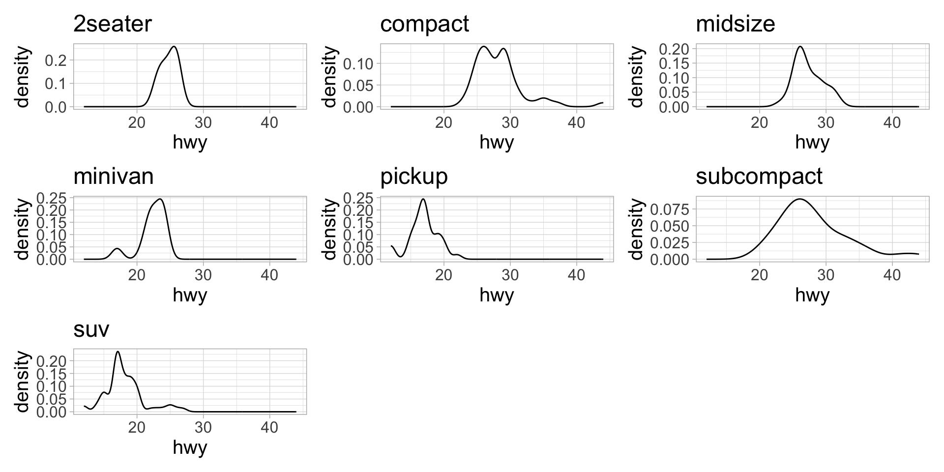
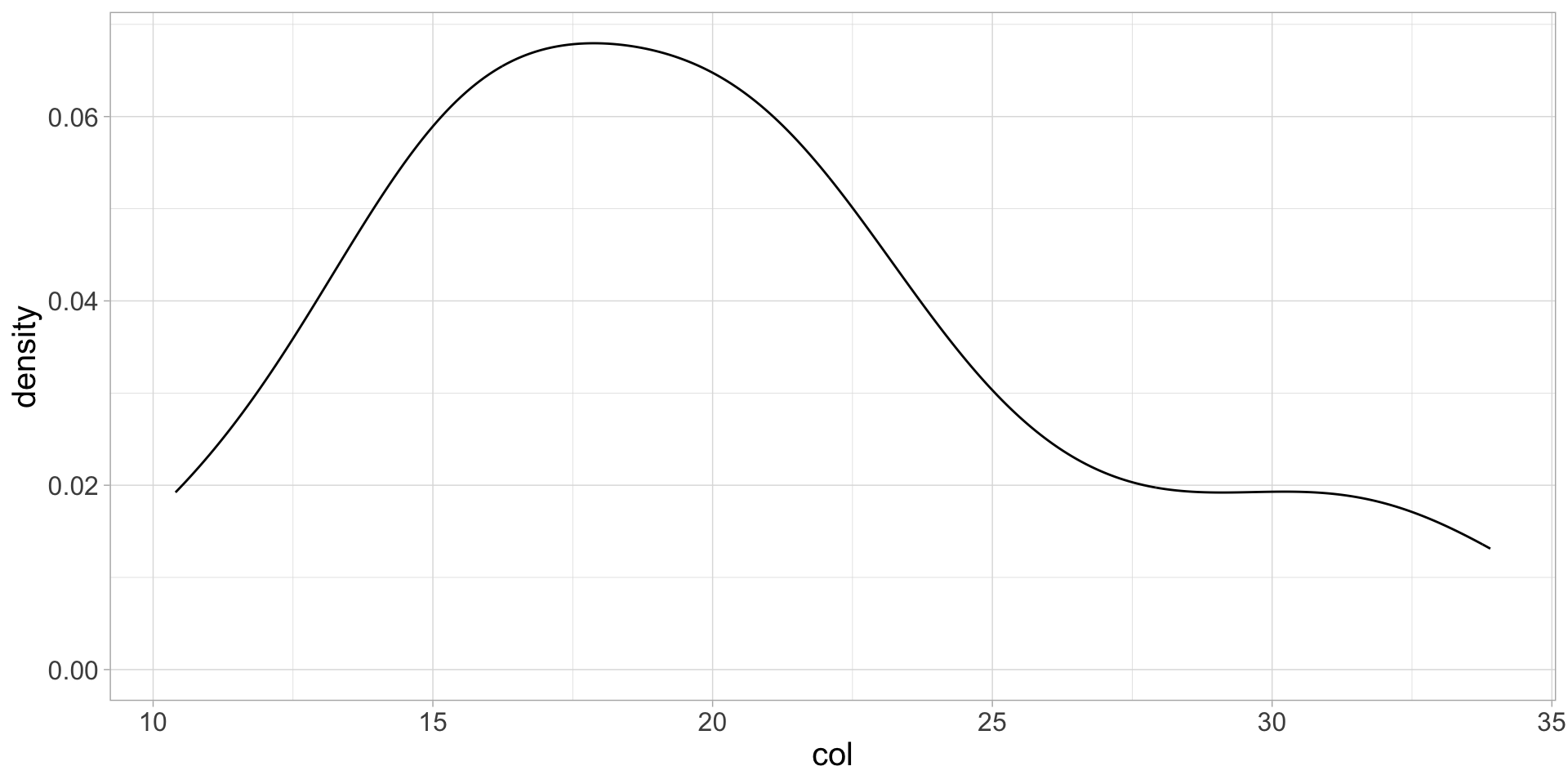
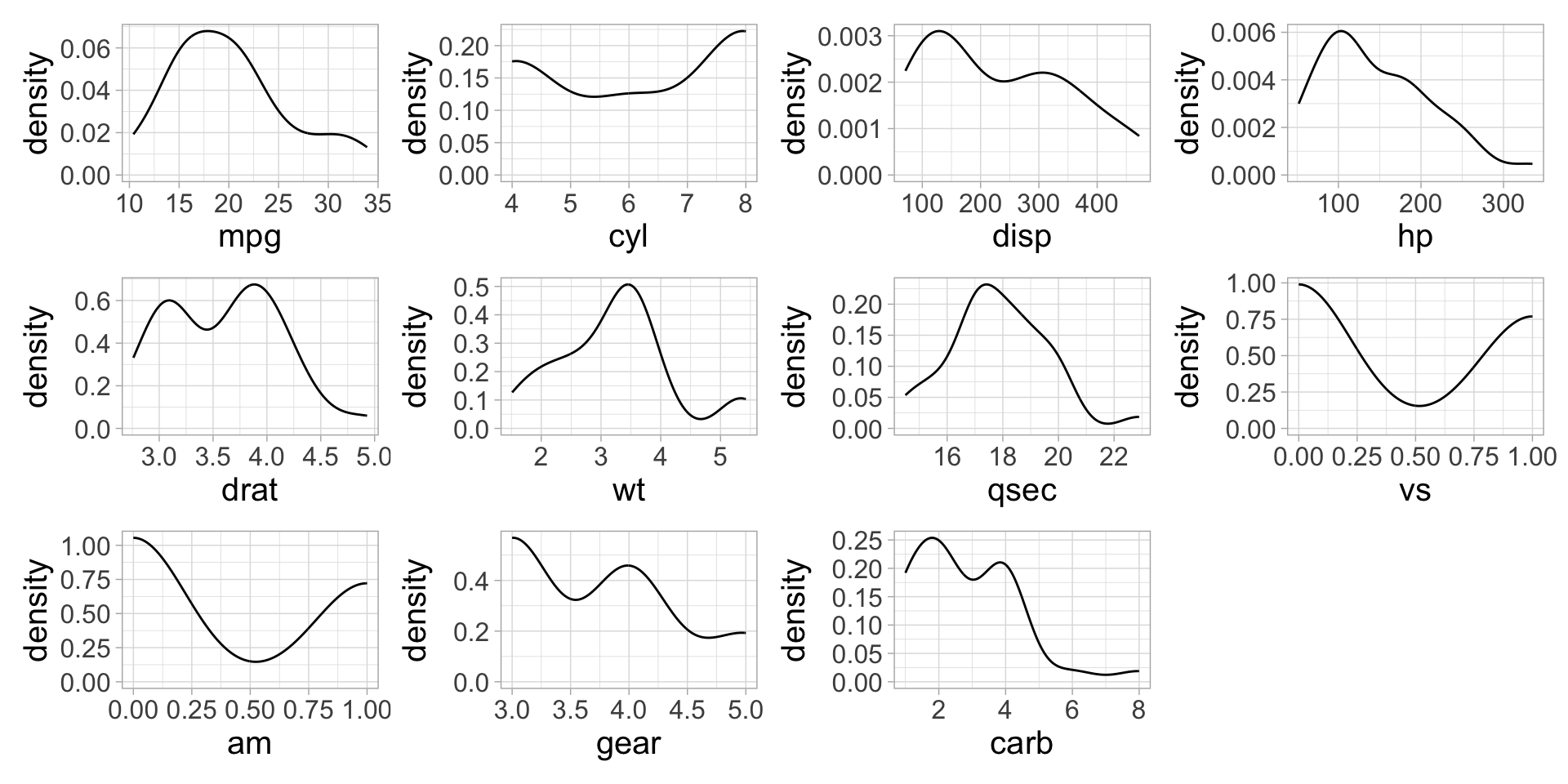
map() over columns to iteratively create plots
- If
map()is supplied with a dataframe, it will iterate over each column. - We need to write a function that takes each column (aka variable) as the argument.
Make it more concise with an anonymous function
Use patchwork::wrap_plots() to view all plots in plot_list
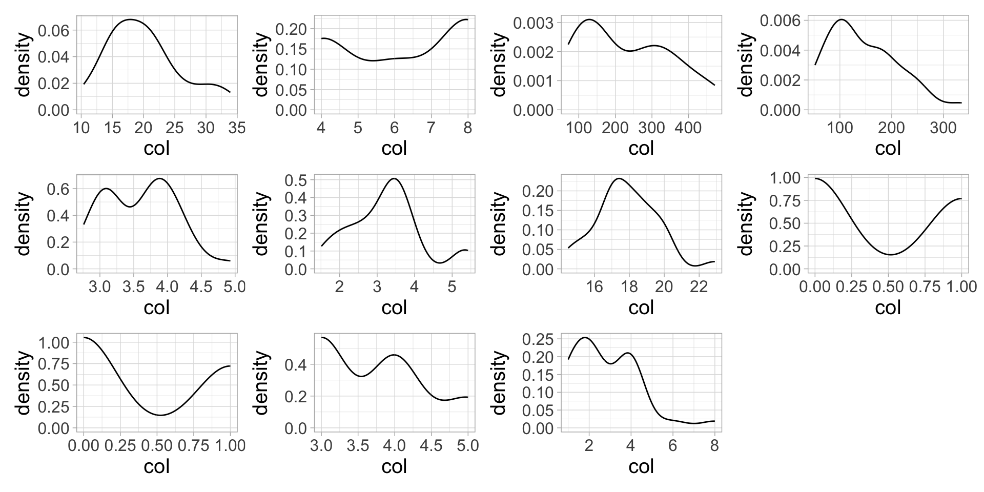
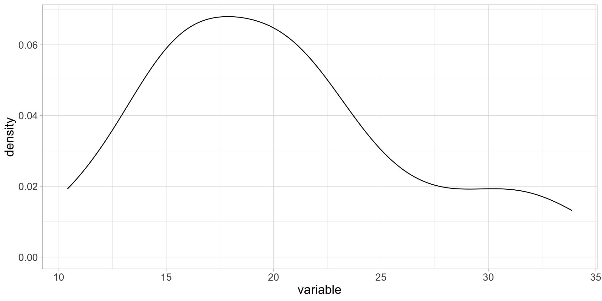
The problem is we don’t know what variables are mapped to the x-axes 😩
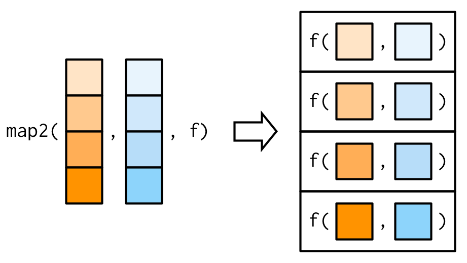
Use map2() when you need to use a function that takes two arguments
Usage:
map2(.x, .y, .f)
.x,.yA pair of vectors, usually the same length.fA function that is takes.xand.yas arguments
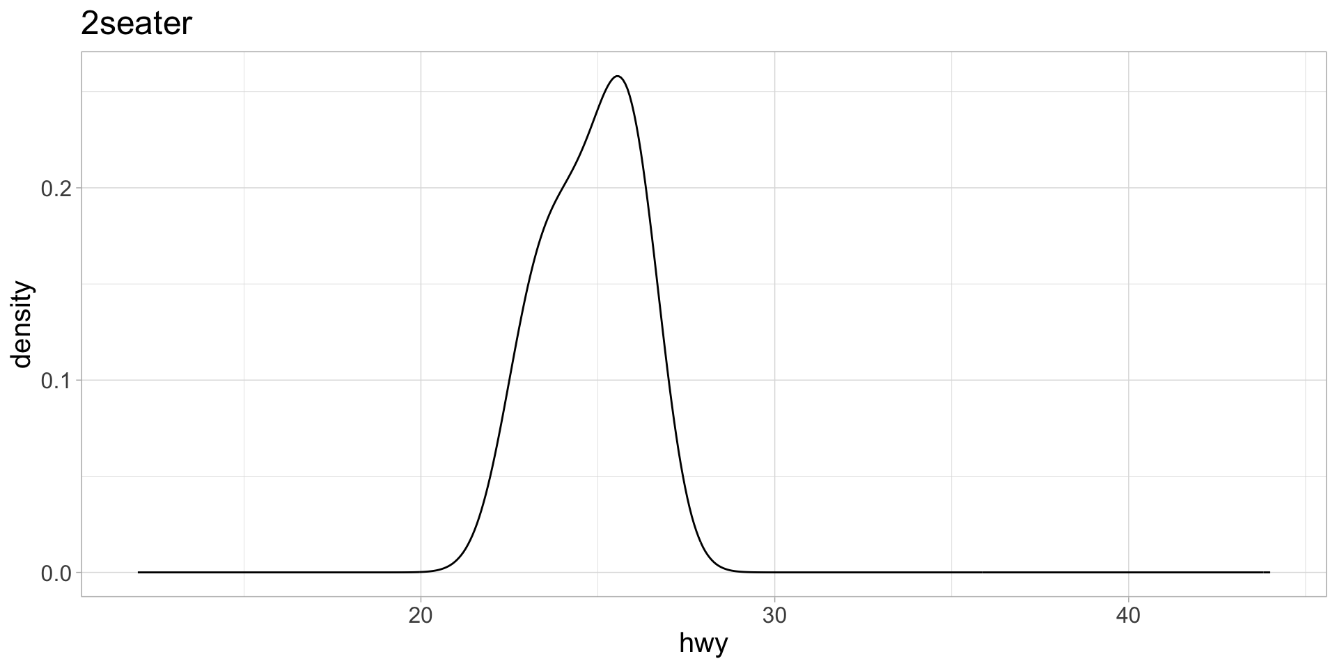
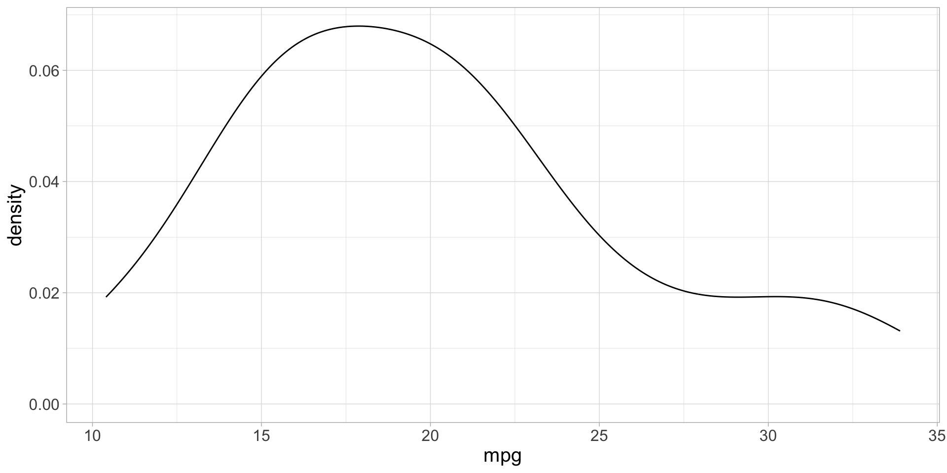
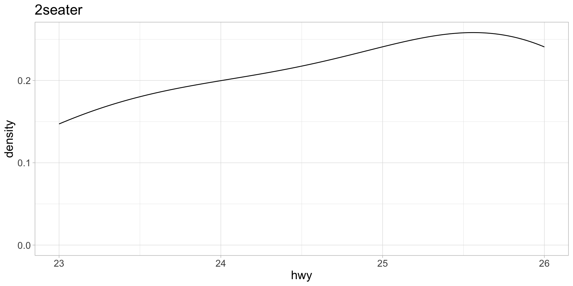
Use map2() to execute the density_plot2() function
Now we have an informative x-axis label!
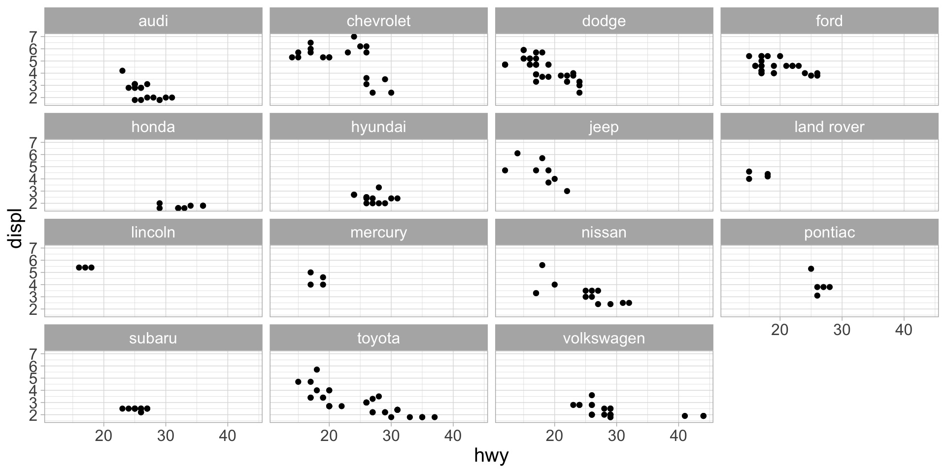
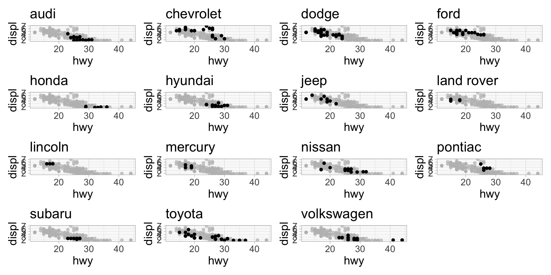
Want: using mpg dataset, plot highway mpg vs displacement, with points highlighted for each manufacturer
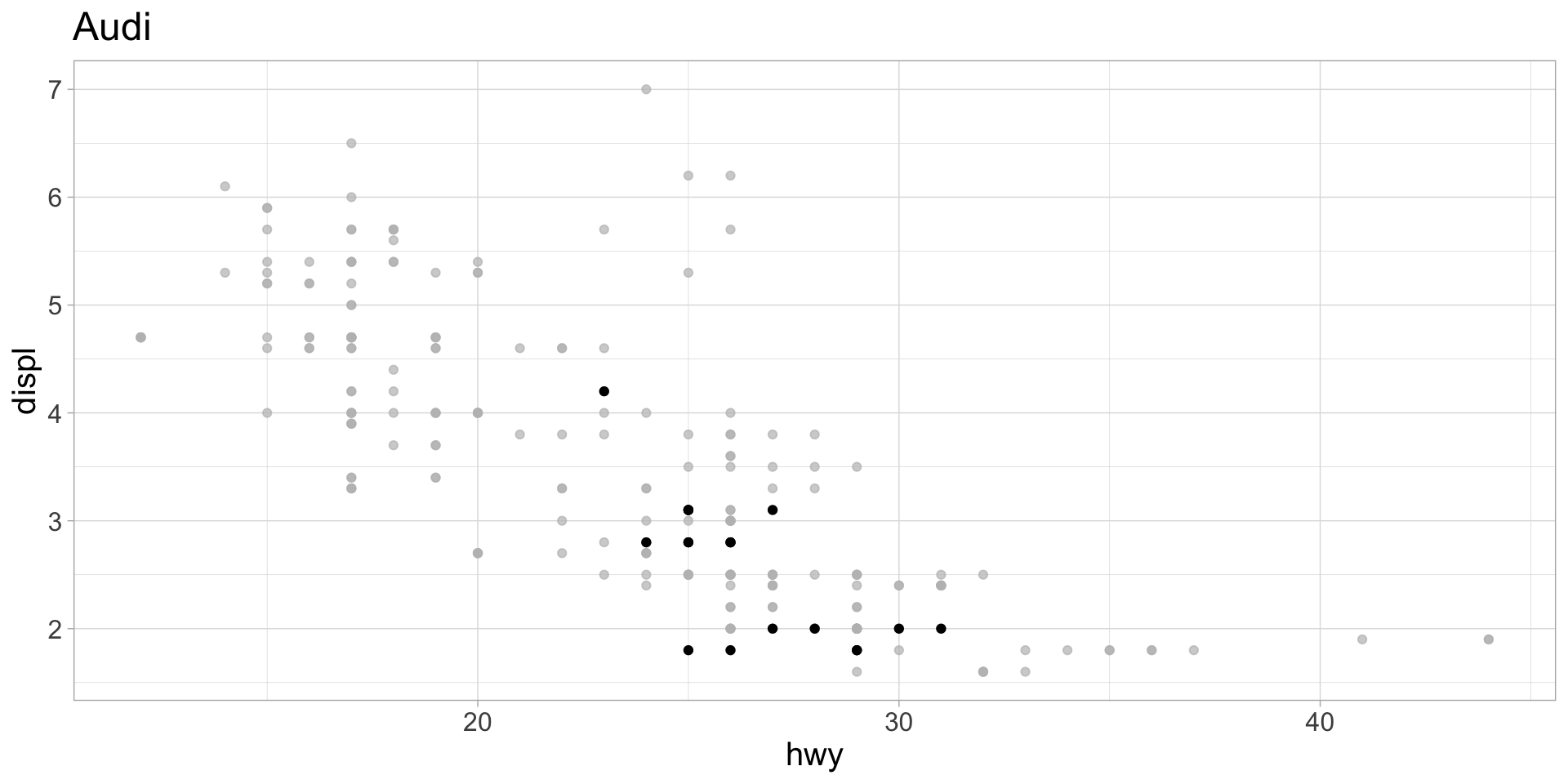
We could facet, but with 15 manufacturers the panels are hard to read and we can’t use the gghighlight function
3. Use map() to execute the function iteratively over each manufacturer. Assign the output to a list called plot_list.
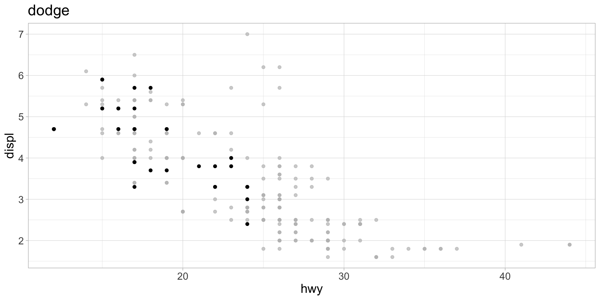
3. map() the function over each data frame in data_list
Check to make sure it worked