Language of models
ENST/MRNE 222 Environmental Data Analysis and Visualization
Statistical modelling
- We use models to explain the relationship between variables and to make predictions
- For now we will focus on linear models (but there are many other types of models too)
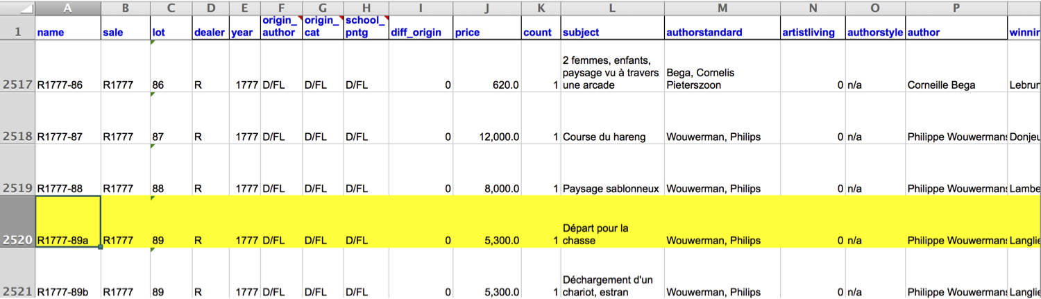
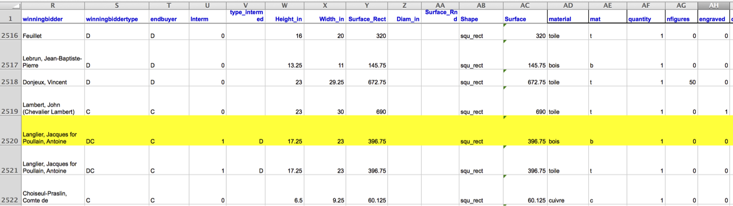
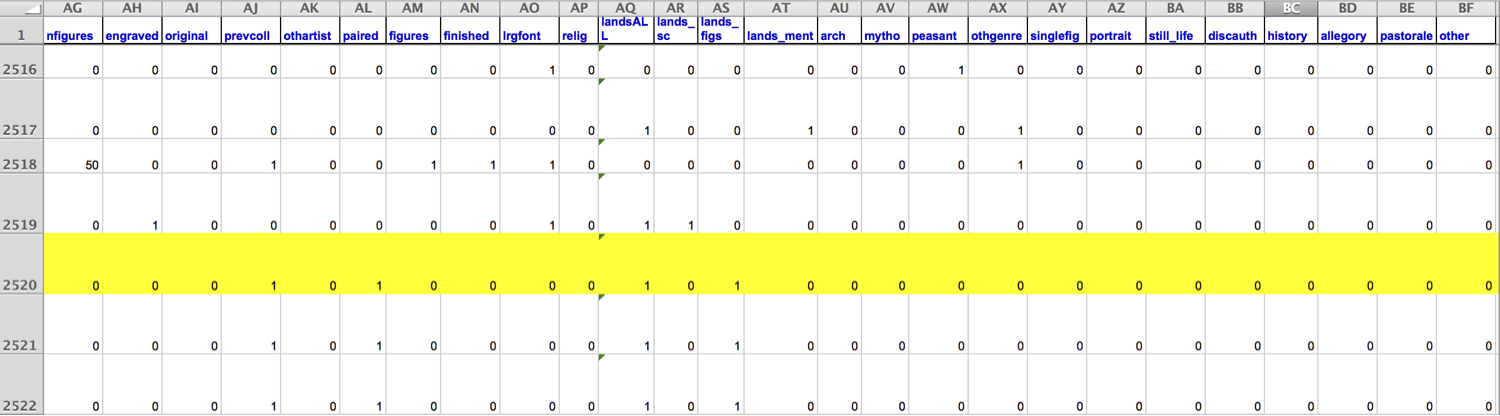
Paris art auction

Data was scraped from auction catalog text
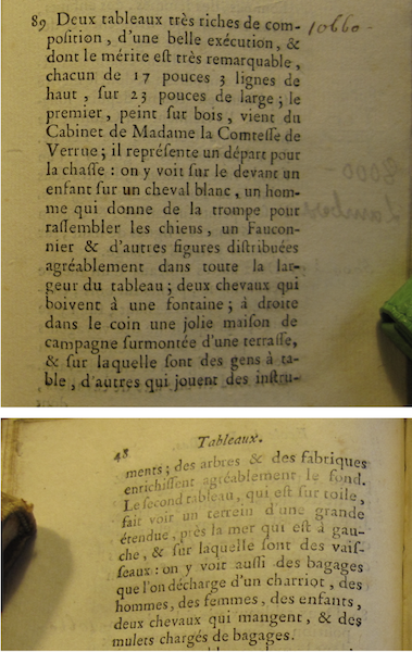
“Two paintings very rich in composition, of a beautiful execution, and whose merit is very remarkable, each 17 inches 3 lines high, 23 inches wide; the first, painted on wood, comes from the Cabinet of Madame la Comtesse de Verrue; it represents a departure for the hunt: it shows in the front a child on a white horse, a man who gives the horn to gather the dogs, a falconer and other figures nicely distributed across the width of the painting; two horses drinking from a fountain; on the right in the corner a lovely country house topped by a terrace, on which people are at the table, others who play instruments; trees and fabriques pleasantly enrich the background.”
Dataset contains numeric and categorical variables
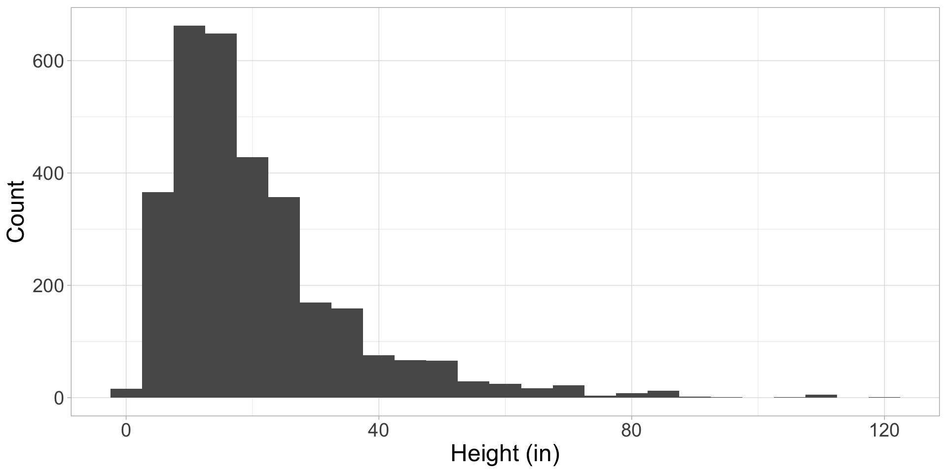
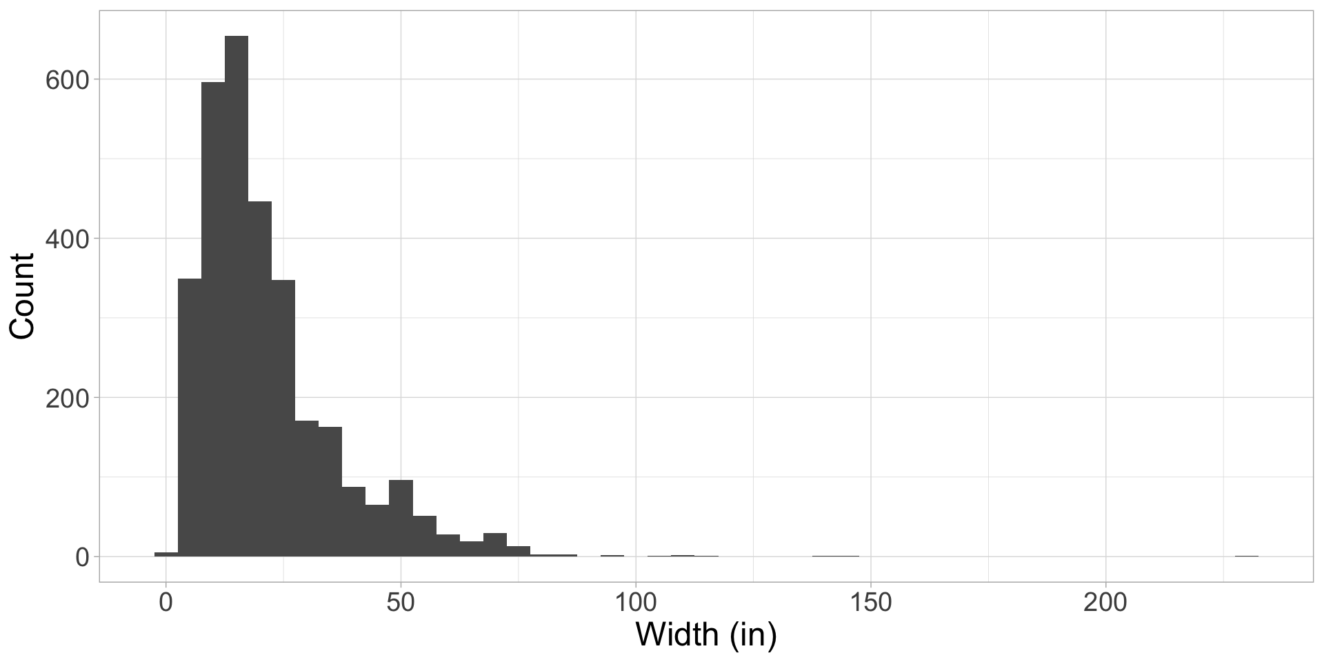
Heights
Widths
Height vs. width
As width increases, height increases:

Height as a function of width
If we know a painting’s width, we can use the equation of the line to calculate the expected height value for a given width.

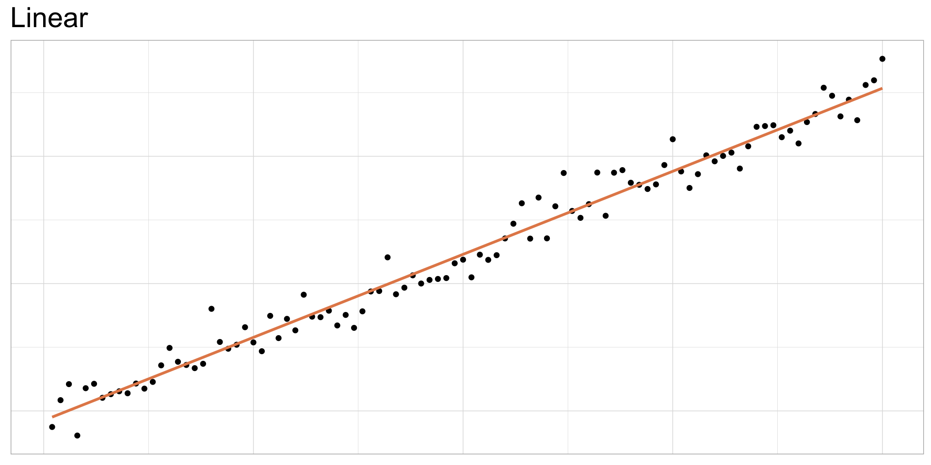
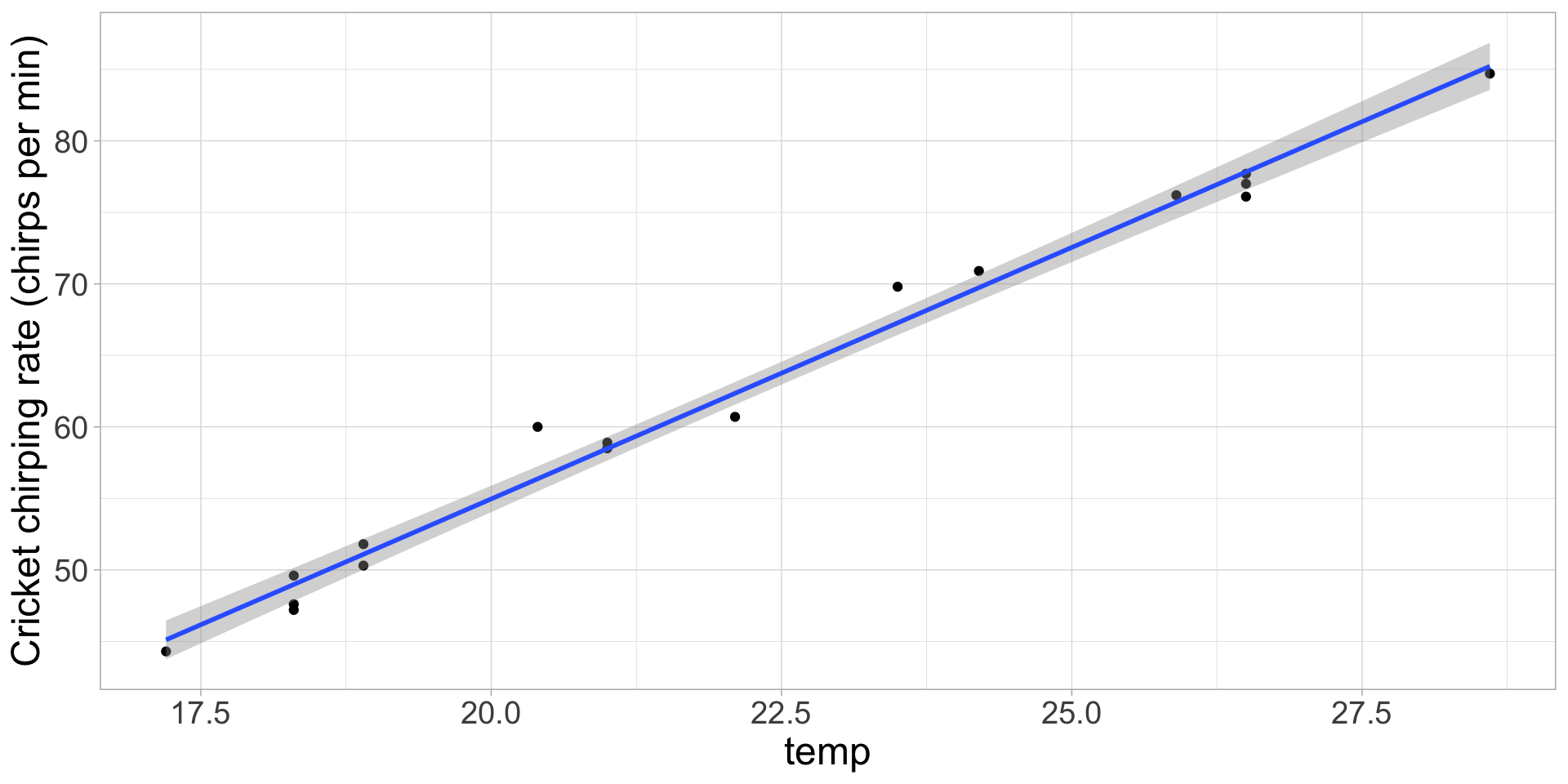
Use geom_smooth(method = "lm") to draw a straight line through your data
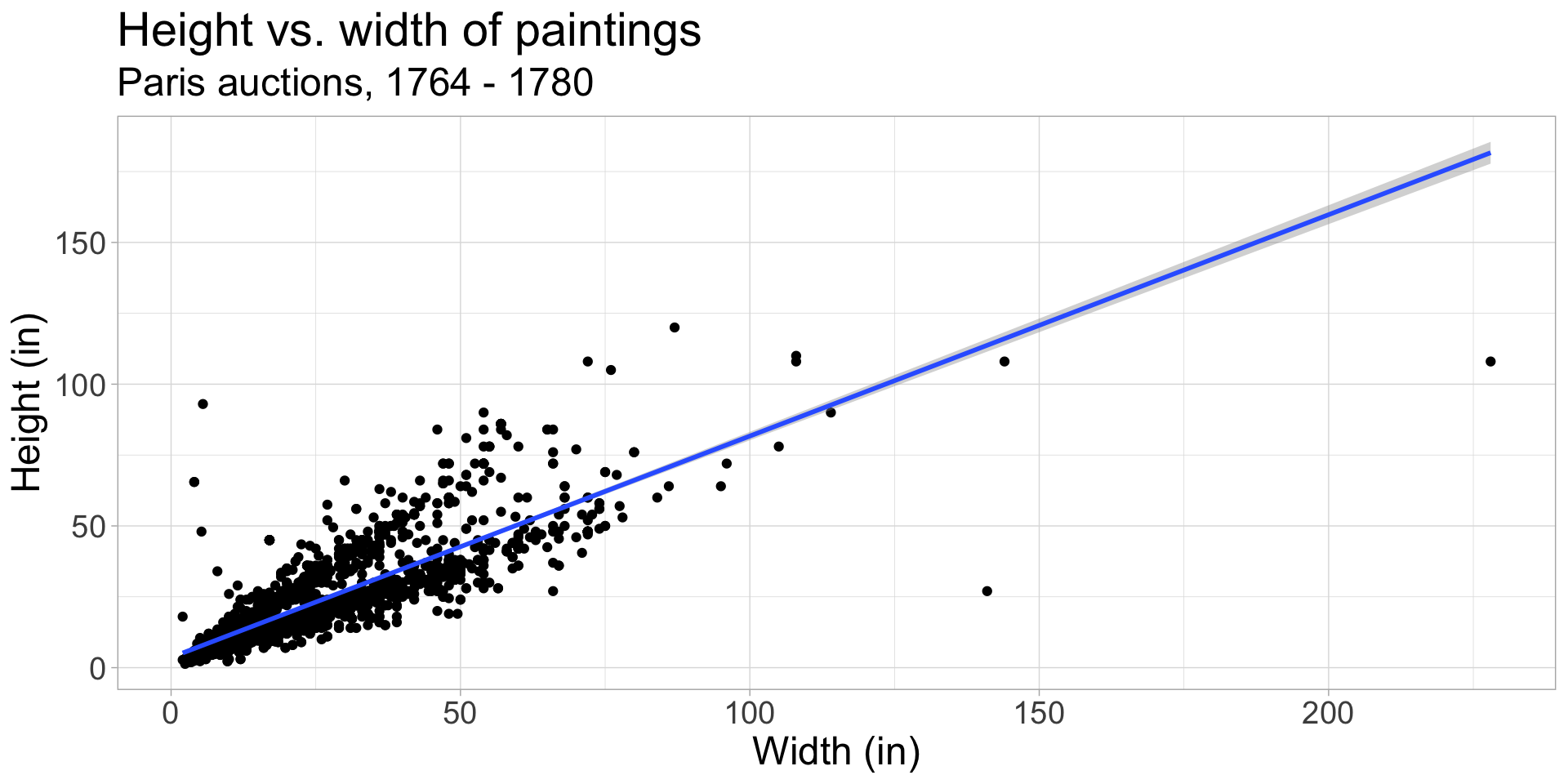
- The gray shading above and below the line represent the confidence interval (CI): the range of values within which the predicted values of y (height) are expected to lie.
- by default,
geom_smooth()uses a 95% CI: 95% percent chance that the actual height is within the range of predicted values in the interval
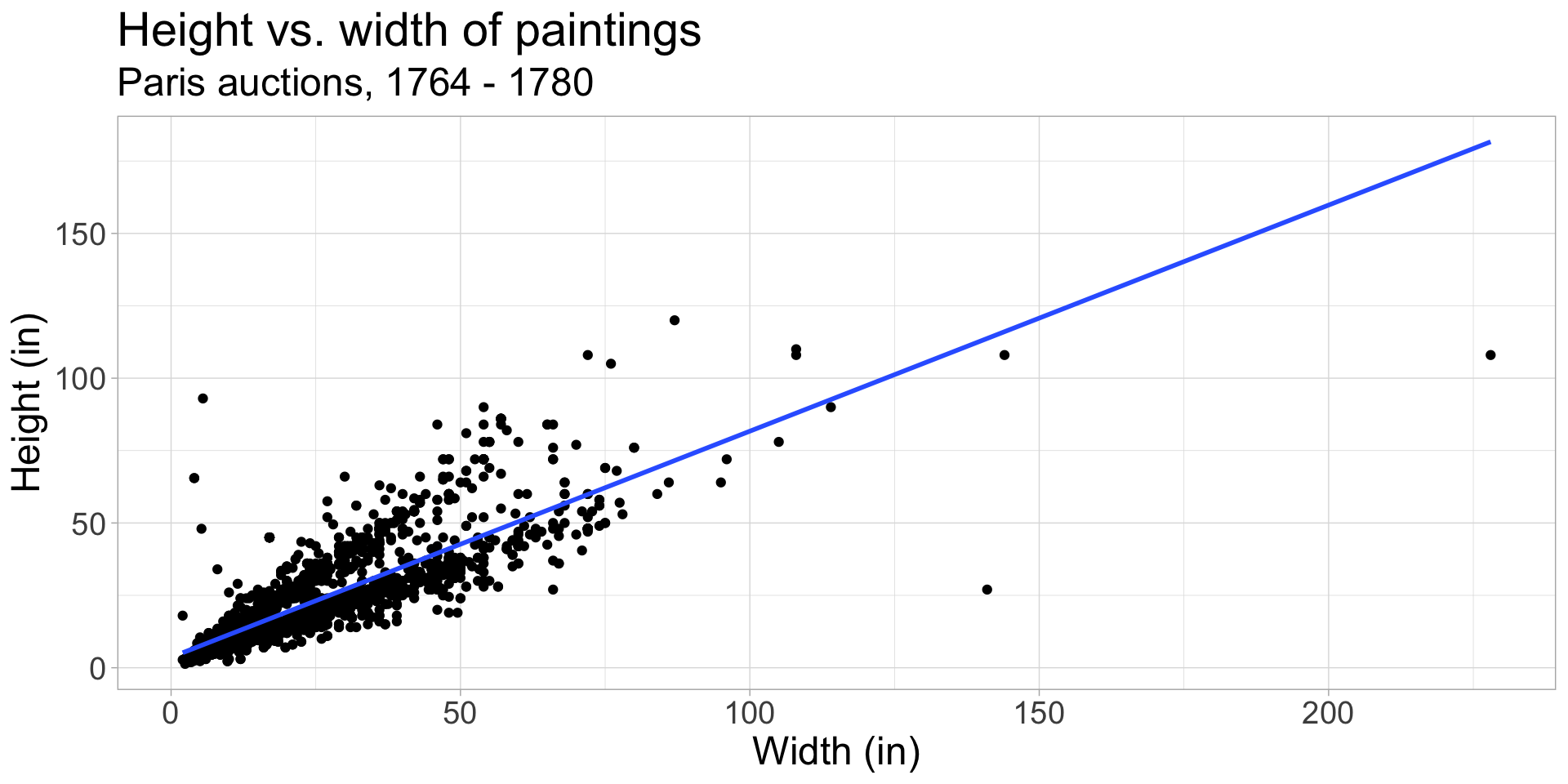
Use geom_smooth(method = "lm", se = FALSE) to remove the CI from the plot
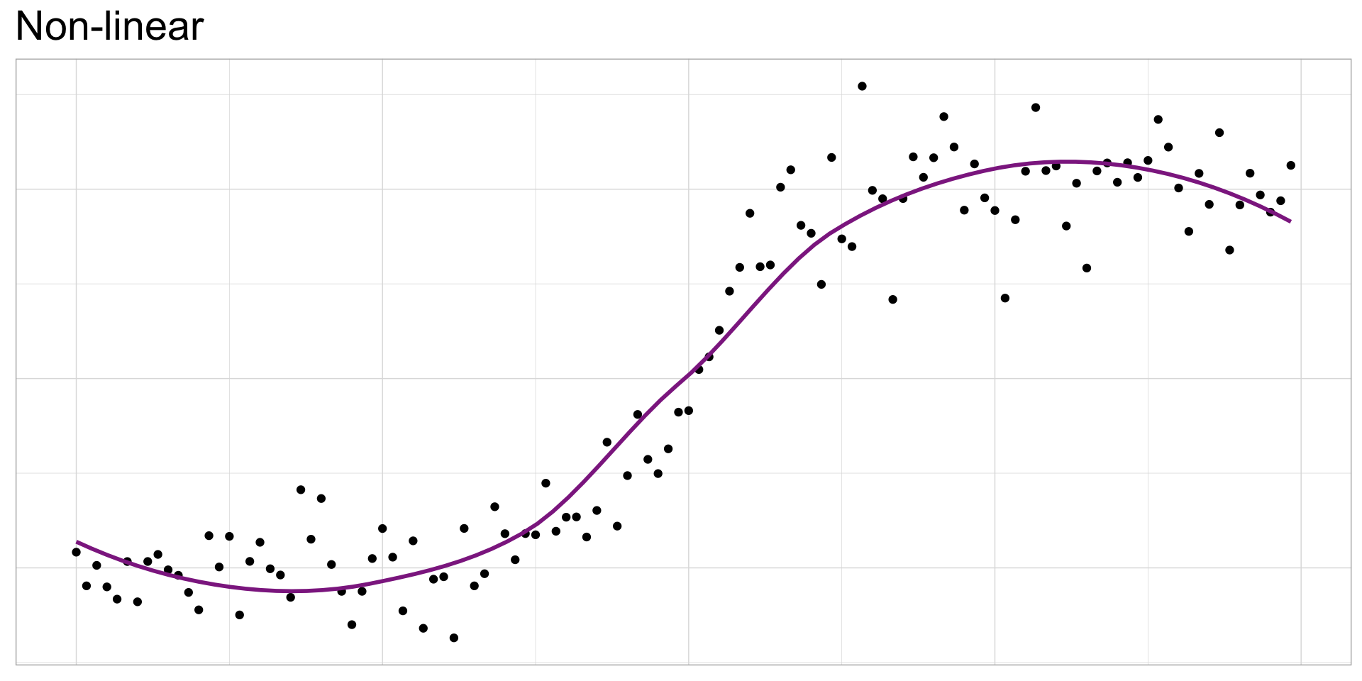
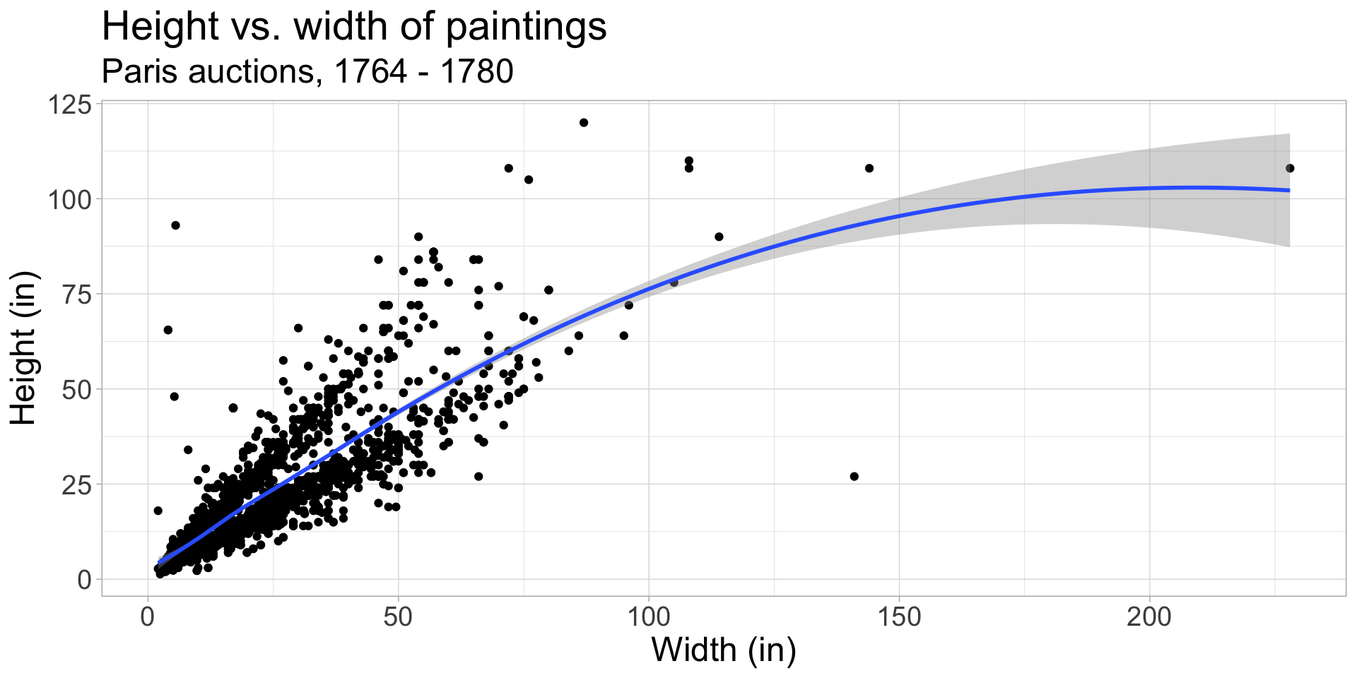
Other smoothing methods: gam
Fits line using a generalized additive model (GAM): allows for non-linear relationships using smoothing functions
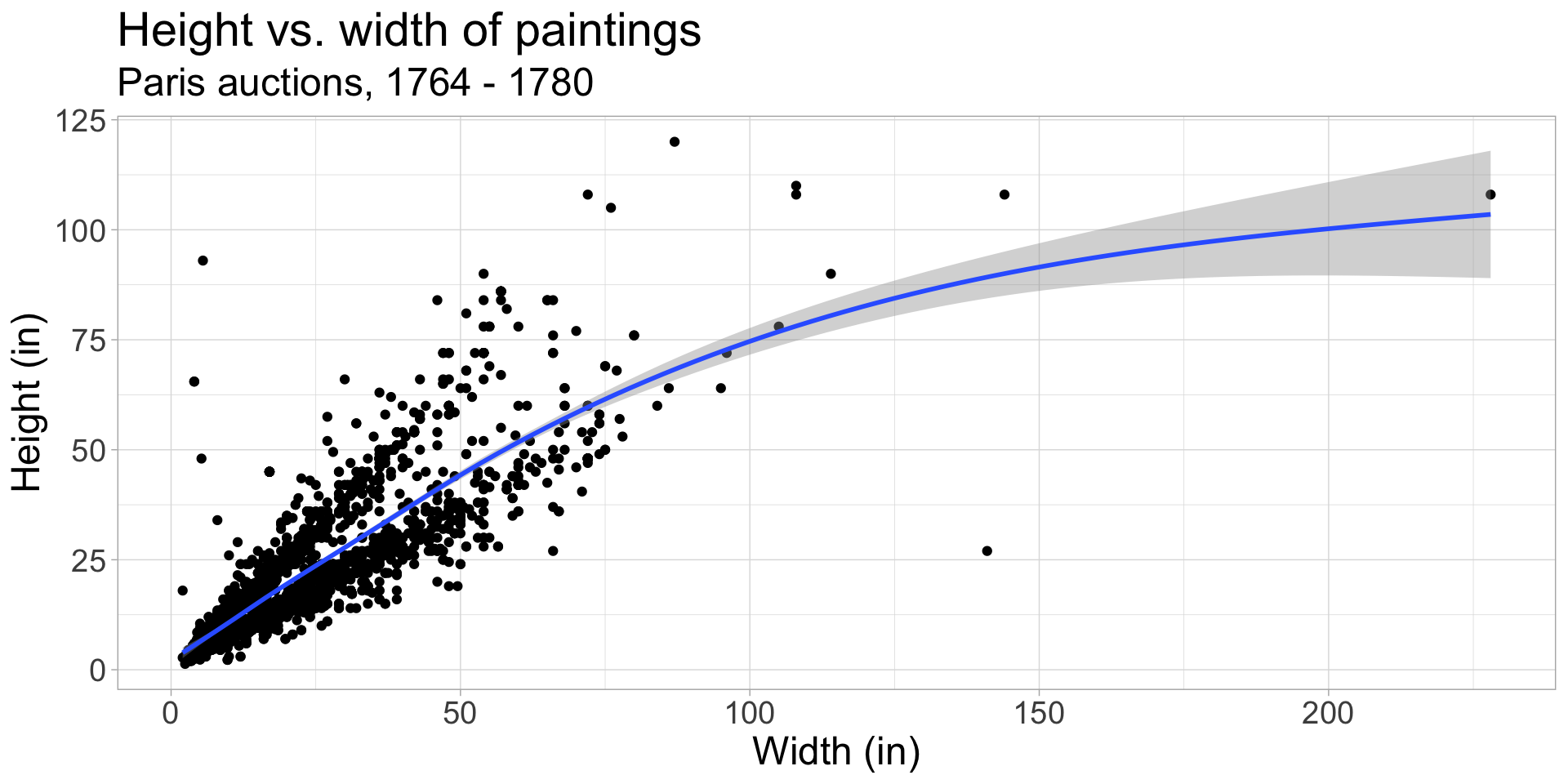
Other smoothing methods: loess
Locally estimated scatterplot smoothing (loess): another method that allows for non-linear relationships
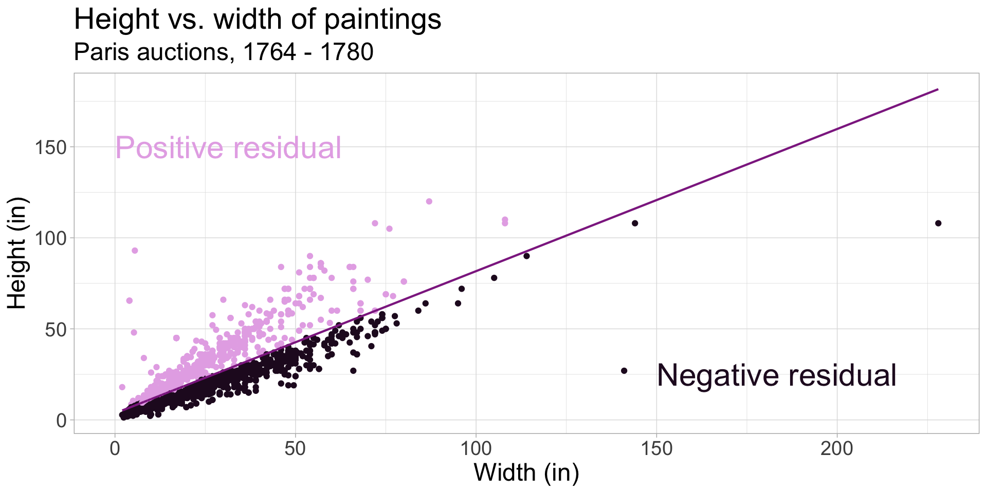
Residuals visualized
ht_wt_fit <- linear_reg() |>
  fit(height_in ~ width_in, data = pp)

ht_wt_fit_tidy <- tidy(ht_wt_fit$fit)
ht_wt_fit_aug  <- augment(ht_wt_fit$fit) |>
  mutate(res_cat = ifelse(.resid > 0, TRUE, FALSE))

ggplot(data = ht_wt_fit_aug) +
  geom_point(aes(x = width_in, y = height_in, color = res_cat)) +
  geom_line(aes(x = width_in, y = .fitted), size = 0.75, color = "#8E2C90") +
  labs(
    title = "Height vs. width of paintings",
    subtitle = "Paris auctions, 1764 - 1780",
    x = "Width (in)",
    y = "Height (in)"
  ) +
  guides(color = FALSE) +
  scale_color_manual(values = c("#260b27", "#e6b0e7")) +
  annotate("text", x = 0, y = 150, label = "Positive residual", color = "#e6b0e7", hjust = 0, size = 8) +
  annotate("text", x = 150, y = 25, label = "Negative residual", color = "#260b27", hjust = 0, size = 8)
Question
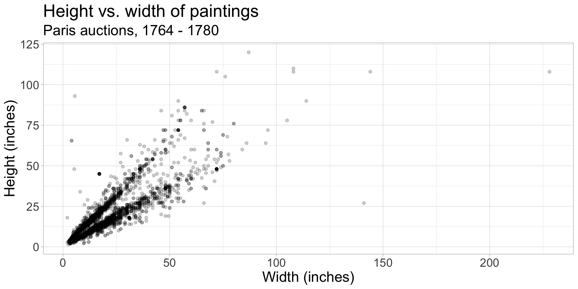
The plot below displays the relationship between height and width of paintings. The only difference from the previous plots is that it uses a smaller alpha value. What feature is apparent now that was not (as) obvious in the previous plots? What might be the reason for this feature?
FYI you can extend regression lines
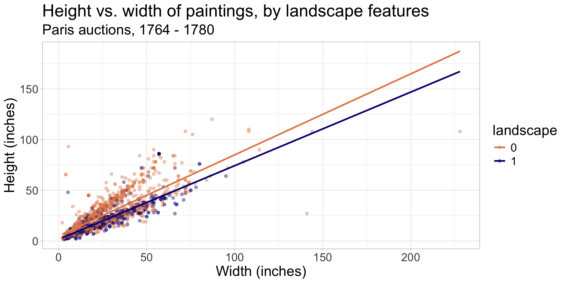
ggplot(data = pp, aes(x = width_in, y = height_in, color = factor(lands_all))) +
  geom_point(alpha = 0.4) +
  geom_smooth(method = "lm", se = FALSE,
              fullrange = TRUE) +
  labs(
    title = "Height vs. width of paintings, by landscape features",
    subtitle = "Paris auctions, 1764 - 1780",
    x = "Width (inches)",
    y = "Height (inches)",
    color = "landscape"
  ) +
scale_color_manual(values = c("#E48957", "#071381"))Slopes vs. differences
Slope: Two numeric variables; for every unit change in x, y changes by … units (the slope gives us …)
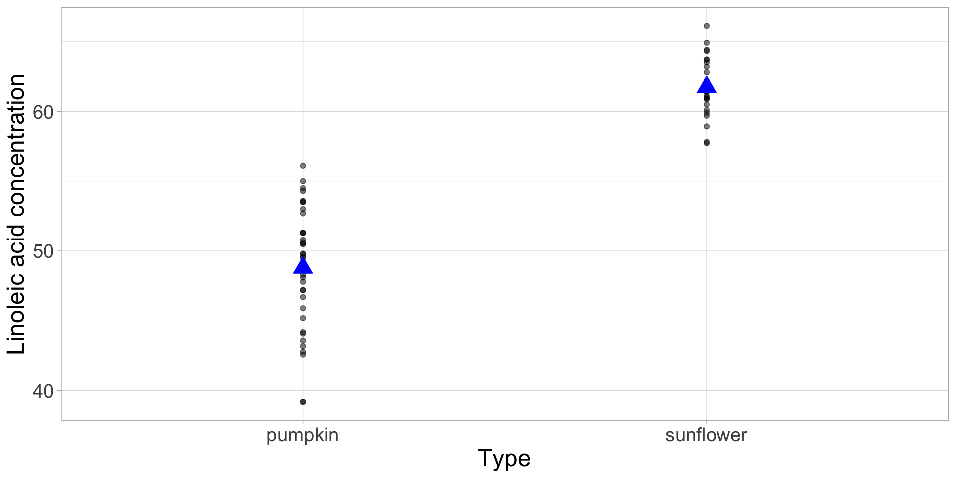
Slopes vs. differences
Difference: 1 numeric, 1 categorical variable; level a of the categorical variable (e.g., pumpkin) is, on average, … units higher/lower than level b of the categorical variable (e.g., sunflower)